Page 64 - IJOCTA-15-4

MN. Khan et.al. / IJOCTA, Vol.15, No.4, pp.594-609 (2025)

1.4
1.2
1
0.8
0.6
0.4
0.2
0
−80 −70 −60 −50 −40 −30 −20 −10 0 10
α
1
1.4
1.2
1
0.8
0.6
0.4
0.2
0
−80 −70 −60 −50 −40 −30 −20 −10 0 10
α
2
6000
5000
4000
3000
2000
1000
0
−80 −70 −60 −50 −40 −30 −20 −10 0 10
α

42
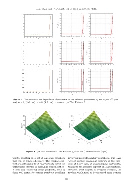
Figure 7. Comparison of the dependence of max-error on the values of parameters α 1 and α 2 with : (1st
row) α 1 = 0, (2nd row) α 2 = 0, (3rd row) α 1 = α 2 = α, of Test Problem 5

20 20
15 15
Solution 10 Solution 10

5 5
0 0
1 1
1 1
0.5 0.5
0.5 0.5
y y x
0 0 x 0 0

Figure 8. 3D view of results of Test Problem 5, exact (left) and numerical (right).

points, resulting in a set of algebraic equations involving integral boundary conditions. The Haar
that can be solved efficiently. The compact sup- wavelet method maintains accuracy in the pres-
port and orthogonality of Haar wavelets have been ence of noisy data or discontinuous coefficients,
particularly effective in managing non-smooth so- thanks to the localized support of Haar functions.
lutions and capturing steep gradients, making However, when applied to irregular domains, the
them well-suited for various parabolic problems method would need to be extended using domain

606