Page 63 - IJOCTA-15-4

Solving parabolic differential equations via Haar wavelets: A focus on integral boundary conditions

8 8

6 6
Solution 4 Solution 4

2 2
0 0
1 1
1 1
0.5 0.5
0.5 0.5
y y x
0 0 x 0 0

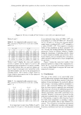
Figure 6. 3D view of results of Test Problem 4, exact (left) and numerical (right)

35
Tables 6 and 7. to an extremely large value of 7.5906 × 10 , cor-
7
responding to a κ value of 7.5623×10 . Moreover,
Table 6. The numerical results generated using for ϑ = 10 and α = 10 the error becomes signifi-
Haar wavelets for Test Problem 5 with dt = 0.0005 180
cantly larger, reaching 4.5071×10 , alongside a
and T = 1 7
κ value of 8.1231 × 10 . This suggests a complete
failure of the simulation at these parameter val-
ϑ = −10 ϑ = 0
α L ∞ κ L ∞ κ ues. Overall, the findings illustrate the impact of
−10 7.8361e − 05 7.6785e + 07 2.3985e − 04 7.5307e + 07 parameter choices on solution behavior, empha-
−03 2.3467e − 04 7.8718e + 07 8.2108e − 05 4.7640e + 07 sizing the importance of selecting suitable values
−02 2.4293e − 04 7.7328e + 07 6.7607e − 05 4.6673e + 07
00 2.6320e − 04 7.5864e + 07 8.5138e − 05 4.2737e + 07 to ensure numerical stability and precision. Addi-
02 2.7061e − 04 7.6323e + 07 3.6215e − 04 4.3677e + 07 tional studies, such as evaluating the convergence
03 2.7821e − 04 7.5311e + 07 2.5000e − 03 4.6090e + 07 of the method, could provide a deeper insight into
10 5.3735e − 04 7.3153e + 07 7.5906e + 35 7.5623e + 07
the problem.
Tables 6 and 7 display the error and condition Figure 7 shows the numerical results of the
number κ against various values of α and ϑ. All proposed method in terms of the comparison be-
simulations used parameters T=1 and dt =0.0005. tween the L ∞ norm and the values of parameters
The results indicate that, as expected, higher val- α 1 and α 2 , while Figure 8 compares the exact and
ues of α lead to increased error variability in the numerical solutions.
non-deterministic case due to the propagation of
rounding errors. For a fixed α, larger values of
ϑ also result in inaccuracies due to the enhanced 5. Conclusions
stiffness phenomenon.
The aim of the article is to numerically solve
partial differential equations with integral bound-
ary conditions using the Haar wavelets collocation
Table 7. The numerical results generated using
Haar wavelets for Test Problem 5 with dt = 0.0005 method. It has investigated the method’s efficacy
and T = 1 and accuracy concerning nonlocal parameters α
and ϑ. The numerical findings have indicated
ϑ = 2 ϑ = 10 that the Haar wavelets approach has performed
α L ∞ κ L ∞ κ effectively and efficiently in addressing parabolic
−50 3.2004e − 04 4.5696e + 08 3.4810e − 04 4.6848e + 08
−30 2.7565e − 04 2.6229e + 08 3.5476e − 04 3.3919e + 08 differential equations with integral boundary con-
−10 2.5726e − 04 5.2507e + 07 7.2413e − 04 8.5954e + 07 ditions, particularly when both α and ϑ have been
−03 2.1362e − 04 4.7381e + 07 3.3986e + 13 7.7049e + 07 negative. However, convergence has failed for the
−02 2.3705e − 04 4.5438e + 07 7.2951e + 19 7.5279e + 07 numerical methods when α and ϑ have exceeded
00 3.6899e − 04 4.3639e + 07 7.7906e + 35 7.2383e + 07
02 5.4200e − 02 4.3476e + 07 6.3430e + 55 7.3907e + 07 3. Maintaining α negative while keeping ϑ posi-
03 4.2767e + 02 4.1867e + 07 2.5365e + 67 7.6128e + 07 tive with equal magnitude or ensuring α magni-
10 6.3430e + 55 7.2669e + 07 4.5071e + 180 8.1231e + 07
tude has been greater than ϑ has enhanced ac-
curacy. The collocation method has guaranteed
It is important to note from Tables 6 and 7, that both the differential equation and integral
that when ϑ = 0 and α = 10, the error escalates boundary conditions have been met at designated
605