Page 61 - IJOCTA-15-4

Solving parabolic differential equations via Haar wavelets: A focus on integral boundary conditions
However, when ϑ reaches 20, there is a notable
increase in the L ∞ norm, which is considerably 1 2 Z 1 κ 2
higher than the error observed for the other ϑ g 2 (t) = − ϑ(κ) dx, (58)
t + 1 0 t + 1
values. Where in Figure 4, the relationship be-
tween ϑ and condition number κ is given. It can
be seen from the figure that the condition num- where, α(κ) = 1 and ϑ(κ) = 1. The theoreti-
ber increases slightly when ϑ increases toward 50 cal solution of this problem is:
from 0. 2
κ
s(κ, t) = . (59)
−5 t + 1
x 10
8.4083
8.4083
8.4083
8.4083
L ∞ 8.4083

8.4083
8.4083
8.4083
8.4083
−50 0 50
ϑ
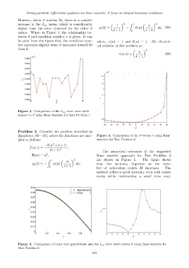
Figure 2. Comparison of the L ∞ error norm with
respect to ϑ using Haar wavelets for Test Problem 1

Problem 3. Consider the problem described by
Equations (20 - 23), where the functions are spec- Figure 4. Comparison of the ϑ versus κ using Haar
ified as follows: wavelets for Test Problem 2
2
−2(κ + t + 1)
f(κ, t) = ,
(t + 1) 3
The numerical outcomes of the suggested
2
ℜ(κ) = κ , Haar wavelet approach for Test Problem 3
Z 1 2 are shown in Figure 5. The figure shows
κ
g 1 (t) = − α(κ) dx, that the accuracy improves as the num-
0 t + 1 ber of collocation points M increases. The
method achieves good accuracy even with coarse
nodes while maintaining a small time step.

0.09
Approximate
0.08 Exact
0.07
0.06
0.05
s
0.04
0.03
0.02
0.01
0
0 0.2 0.4 0.6 0.8 1
x
Figure 3. Comparison of exact and approximate and the L ∞ error norm versus ϑ using Haar wavelets for
Test Problem 2
603