Page 51 - IJPS-1-1

Giambattista Salinari and Gustavo De Santis

ln µ , c x lnα = c β + x ν + , c x x k= 0 + 1, ,75

with the new error terms ν , c x .
Differentiating by age yields a new set of series δ x:

δ , c x = ln(µ , c x+ 1 ) ln(µ − , c x )
which by assumption, will oscillate around zero until age k 0 and around β after age k 0,
where β is the slope of the log force of mortality:
δ , c x = 0 ω + , c x x = 25,26, ,k 0 . (3)

δ = βω+ x k= + 1, ,75
, c x , c x 0
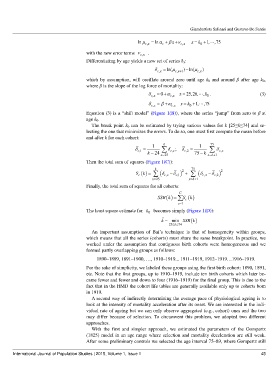
Equation (3) is a “shift model” (Figure 1(B)), where the series “jump” from zero to β at
age k 0.
The break point k 0 can be estimated by trying various values for k [25≤k≤74] and se-
lecting the one that minimizes the errors. To do so, one must first compute the mean before
and after k for each cohort:
1 k 1 75
∑
∑
δ c ,1 = k − 24 x= 25 δ , c x ; δ c ,2 = 75 k x k+ 1 δ , c x
−
=
Then the total sum of squares (Figure 1(C)):
k 2 75 2
Sk ∑ ( c ,x − δ c ,1 ) + ∑ ( c ,x − δ c ,2 )
δ
δ
( ) =
c
=
x= 25 x k+ 1
Finally, the total sum of squares for all cohorts:
C
SSR ( ) k = ∑ S c ( ) k
c= 1
The least square estimate for k becomes simply (Figure 1(D)):
0
ˆ
k = min SSR ( ) k
25 k≤≤ 74
An important assumption of Bai’s technique is that of homogeneity within groups,
which means that all the series (cohorts) must share the same breakpoint. In practice, we
worked under the assumption that contiguous birth cohorts were homogeneous and we
formed partly overlapping groups as follows:
1890–1899, 1891–1900, …, 1910–1919... 1911–1919, 1912–1919…1916–1919.
For the sake of simplicity, we labeled these groups using the first birth cohort: 1890, 1891,
etc. Note that the first groups, up to 1910–1919, include ten birth cohorts which later be-
came fewer and fewer and down to four (1916–1919) for the final group. This is due to the
fact that in the HMD the cohort life tables are generally available only up to cohorts born
in 1919.
A second way of indirectly determining the average pace of physiological ageing is to
look at the intensity of mortality acceleration after its onset. We are interested in the indi-
vidual rate of ageing but we can only observe aggregated (e.g., cohort) ones and the two
may differ because of selection. To circumvent this problem, we adopted two different
approaches.
With the first and simpler approach, we estimated the parameters of the Gompertz
(1825) model in an age range where selection and mortality deceleration are still weak.
After some preliminary controls we selected the age interval 75–89, where Gompertz still

International Journal of Population Studies | 2015, Volume 1, Issue 1 45