Page 131 - IJPS-11-5

International Journal of
Population Studies Regional disparities and fertility rates

was expected to identify not only the influence of widening 3. Results
regional disparities on the fertility rate over time but also
to forecast future fertility rate trends. 3.1. Bivariate model
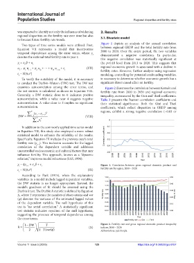
Two types of time series models were utilized. First, Figure 1 depicts an analysis of the annual correlation
Equation VII represents a model that incorporates between regional GRDP and the total fertility rate from
temporal dependence among the error terms, where y t 2000 to 2020. Over the entire period, the two variables
denotes the national total fertility rate in year t. demonstrated a negative correlation. In particular,
this negative correlation was statistically significant at
y = x β + u the p<0.10 level from 2013 to 2020. This suggests that
t t t
u = ψ u + ψ u + ⋯ + ψ u + ε (VII) regional economic growth is associated with a decline in
t 1 t−1 2 t2 m t−m t fertility rates. However, further analysis using regression
ε ~ N(0,σ )
2
t modeling, controlling for potential confounding variables,
To verify the suitability of the model, it is necessary is necessary to determine whether economic growth has a
to conduct the Durbin–Watson (DW) test. The DW test significant direct causal effect on fertility.
examines autocorrelation among the error terms, and Figure 2 illustrates the correlation between Korea’s total
the test statistic is calculated as shown in Equation VIII. fertility rate from 2000 to 2020 and regional economic
Generally, a DW statistic close to 0 indicates positive inequality, as measured by the Gini and Theil coefficients.
autocorrelation, while a value near 4 suggests negative Table 3 presents the Pearson correlation coefficients and
autocorrelation. A value close to 2 implies no significant their statistical significance. Both the Gini and Theil
autocorrelation. coefficients, which reflect disparities in GRDP among
∑ T (ε −ε ) 2 regions, exhibit a strong negative correlation (−0.83 or
DW = t =2 t t −1 (VIII)
∑ T t =1 ε t 2 0

In addition to the commonly applied time series model -0.1
in Equation VII, this study also employed a more robust -0.2
statistical model to enhance the reliability of the results. Correlation coefficient
Specifically, Equation IX includes the previous year’s total -0.3
fertility rate (y ). This inclusion accounts for the lagged
t−1
correlation of the dependent variable and addresses -0.4
uncontrolled socioeconomic and cultural factors that may -0.5
influence fertility. This approach, known as a “dynamic 2000 2002 2004 2006 2008 2010 2012 2014 2016 2018 2020
solution,” improves model robustness (SAS, 1996). Year
y = ϕy + x β + ε t Figure 1. Correlation between gross regional domestic product and
t
t−1
t
ε ~ N(0,σ ) (IX) fertility rate by region, 2000 – 2020
2
t
According to Park (1975), when the explanatory
variables in a model include lagged dependent variables, 1.60 0.50
the DW statistic is no longer appropriate. Instead, the 1.40 0.40
model’s goodness of fit should be assessed using the 1.20
Durbin h test. The Durbin h statistic is defined by Equation 1.00 0.30
X, where T represents the number of observations and var Fertility rate 0.80 Gini & Theil
(φ) denotes the variance of the estimated lagged values 0.60 0.20
of the dependent variable. The null hypothesis of this 0.40 0.10
test is “no serial correlation.” A statistically significant 0.20
test statistic indicates rejection of the null hypothesis, 0.00 0.00
suggesting the presence of temporal dependence among 2000 2001 2002 2003 2004 2005 2006 2007 2008 2009 2010 2011 2012 2013 2014 2015 2016 2017 2018 2019 2020
the error terms. Fertility rate Year Gini Theil

1 − DW  T Figure 2. Fertility rate and gross regional domestic product inequality
h =   (X) indices, 2000 – 2020
Tvar( )φ
 2  1 − ( Abbreviation: ppl: People.

Volume 11 Issue 5 (2025) 125 https://doi.org/10.36922/ijps.8157