Page 130 - IJPS-11-5

International Journal of
Population Studies Regional disparities and fertility rates

independent variables. In addition, it enables the The SEM, unlike the SAR model, assumes the presence
identification of variations over time (Hsiao, 2014; Lee of spatial dependence in the error term rather than in the
& Noh, 2012). Applying traditional econometric models dependent variable. represents the spatial autocorrelation
that do not consider spatial dependency or spatial coefficient, indicating spatial autocorrelation among the
autocorrelation in regional studies may have a negative error terms.
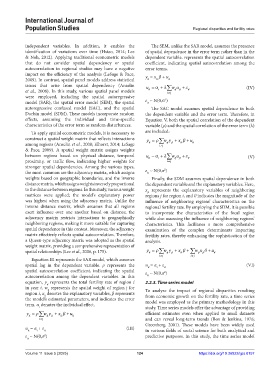
impact on the efficiency of the analysis (LeSage & Pace, y = x β + u
2009). In contrast, spatial panel models address statistical it it it
issues that arise from spatial dependency (Anselin u =α + λ ∑ w u +ε (IV)
et al., 2008). In this study, various spatial panel models it i ij ij jt it
≠
were employed, including the spatial autoregressive 2
model (SAR), the spatial error model (SEM), the spatial ε ~ N(0,σ )
it
autoregressive confused model (SAC), and the spatial The SAC model assumes spatial dependence in both
Durbin model (SDM). These models incorporate random the dependent variable and the error term. Therefore, in
effects, assuming the individual and time-specific Equation V, both the spatial correlation of the dependent
characteristics of the error term as random disturbances. variable (ρ) and the spatial correlation of the error term (λ)
To apply spatial econometric models, it is necessary to are included:
construct a spatial weight matrix that reflects interactions y = ρ ∑ w y + x β + u
among regions (Anselin et al., 2008; Elhorst, 2014; LeSage it ij ij jt it it
≠
& Pace, 2009). A spatial weight matrix assigns weights
between regions based on physical distance, temporal u =α i + λ ∑ w u +ε it (V)
it
jt
ij
proximity, or traffic flow, indicating higher weights for ij
≠
stronger spatial dependencies. Among the various types, 2
the most common are the adjacency matrix, which assigns ε ~ N(0,σ )
it
weights based on geographic boundaries, and the inverse Finally, the SDM assumes spatial dependence in both
distance matrix, which assigns weights inversely proportional the dependent variable and the explanatory variables. Here,
to the distance between regions. In this study, various weight x represents the explanatory variables of neighboring
jt
matrices were applied; the model’s explanatory power regions j for region i, and θ indicates the magnitude of the
was highest when using the adjacency matrix. Unlike the influence of neighboring regions’ characteristics on the
inverse distance matrix, which assumes that all regions regional fertility rate. By employing the SDM, it is possible
exert influence over one another based on distance, the to incorporate the characteristics of the focal region
adjacency matrix restricts interactions to geographically while also assessing the influence of neighboring regions’
neighboring regions, making it more suitable for capturing characteristics. This facilitates a more comprehensive
spatial dependence in this context. Moreover, the adjacency examination of the complex determinants impacting
matrix effectively reflects spatial autocorrelation. Therefore, fertility rates, thereby enhancing the sophistication of the
a Queen-type adjacency matrix was adopted as the spatial analysis.
weight matrix, providing a comprehensive representation of
spatial relationships (Lee et al., 2006, p. 175). y = ρ ∑ w y + x β + ∑ wx θ + u it
it
ij
it
ij
jt
jt
≠
ij ij
≠
Equation III represents the SAR model, which assumes
spatial lag in the dependent variable. ρ represents the u = α + ε it (VI)
i
it
spatial autocorrelation coefficient, indicating the spatial ε ~ N(0,σ )
2
autocorrelation among the dependent variables. In this it
equation, y represents the total fertility rate of region i 2.2.3. Time series model
it
in year t, w represents the spatial weight of region j for To analyze the impact of regional disparities resulting
ij
region i, x denotes the explanatory variables, β represents from economic growth on the fertility rate, a time series
it
the model’s estimated parameters, and indicates the error model was employed as the primary methodology in this
term. α denotes the individual effect. study. Time series models offer the advantage of providing
i
y = ρ ∑ w y + x β + u it efficient estimates even when applied to small datasets
it
jt
ij
it
≠
ij and can reveal long-term trends (Box & Jenkins, 1976;
Greenberg, 2001). These models have been widely used
u = α + ε it (III) in various fields of social science for both analytical and
i
it
ε ~ N(0,σ ) predictive purposes. In this study, the time series model
2
it
Volume 11 Issue 5 (2025) 124 https://doi.org/10.36922/ijps.8157