Page 49 - IJPS-5-1

Mirembe, et al.

half (50.9%) of the sample had a child, 71.3% had secondary or more education while 28.7% had primary or low-level
educational attainment. More than half (54.8%) of the sample had never been married while only 27.0% were married.
A majority (77.4%) of the sample did not belong to any social network, 79.5% of the migrants had left their places of
origin due to economic reasons, and 24.8% of the migrants were residing in Kampala region.

3.1. Associates of Migration Status
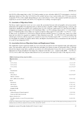
The binary logistic regression model was run to assess the association between both demographic and socioeconomic
individual-level variables with migration status, as shown in Table 2. Results in Table 2 showed that age, residence, and
region had a significant association with migration status (p<0.05). With age, youths aged 23-27 had increased odds to
be migrants as compared to those aged 18-22 (Odds Ratio [OR] = 1.4; 95% confidence interval [CI]: 1.0-1.8) and youths
aged 33-35 had almost three more odds to be migrants compared to those aged 18-22 years (OR = 2.5; 95% CI: 1.3-4.5).
In other words, the likelihood of youth being a migrant increased with the increase in a youth’s age. Youths from urban
areas had less odds to be migrants as compared to those from rural areas (OR = 0.4, 95% CI: 0.3-0.6) and youths from
central region had more odds be migrants as compared to those from Northern region (OR = 1.0; 95% CI: 0.5-1.0). On
the other hand, sex, number of children, marital status, and highest education level had no association with the likelihood
of a youth being a migrant (p>0.05).

3.2. Association between Migration Status and Employment Status
The multinomial logistic regression model was run to assess the association between migration status and employment
status. This association could not be tested with other individual level factors because of collinearity (Table 3). Results
showed that migrant status had a significant association with self-employment because the risk of a youth being self-
employed over being unemployed was higher for a migrant youth than a non - migrant youth (RRR = 1.4, 95% CI:
1.0-2.0). On the other hand, migrant status did not have any association with employed status of the migrant (p>0.05).

Table 2. Factors predicting migration status.
Migration status Odds ratio
Age
23-27 (18-22) 1.4 (1.0-1.8)*
28-32 (18-22) 1.5 (1.0-2.2)
33-35 (18-22) 2.5 (1.4-4.5)**
Sex
Female (Male) 1.1 (0.9-1.5)
Residence
Urban (Rural) 0.4 (0.3-0.6)**
Number of children
Have a child and more (None) 0.9 (0.6-1.2)
Region
East (North) 0.7 (0.5-1.1)
West (North) 0.7 (0.5-1.0)
Central (North) 1.0 (0.5-1.0)*
Kampala (North) 1.0 (0.7-1.4)
Marital status
Widowed/Separated (Currently married) 1.2 (0.8-1.8)
Never married (Currently married) 0.9 (0.6-1.3)
Highest education level
Secondary education or more (Primary education or 0.6 (0.4-0.8)
lower)
(1) There were 1524 observations. (2) The category of a variable in the parentheses is the reference group of the variable. (3) ORs (odds ratios) in the parentheses are the 95%
confidence intervals. All ORs were adjusted for covariates in Table 1. (4) *p<0.05, **p=0.01.

International Journal of Population Studies | 2019, Volume 5, Issue 1 43