Page 118 - MSAM-3-2

Materials Science in Additive Manufacturing Hybrid lattice structures design with AI

A where l is the layer number, A is the activation signal, Z
is the output signal, W is the weight, b is the bias, and f is
the activation function of a given layer.
Rectified linear unit (ReLU) activation function was
used for each neuron:

x + x   xifx > 0
fx + = max (0,x ) = = 
( ) = x
2   0otherwise (XVI)
B
where x represents the input to the neuron.
To enhance generalization and mitigate overfitting, dropout
layers were strategically positioned between dense layers, with
dropout rates of 30% and 20%. The output layer comprises four
neurons with a linear activation function, which quantifies
E , E , ν and ν of the hybrid lattice. The model was trained
y
yx
x
xy
utilizing the mean squared error (MSE) loss function:
2
 ( ) i ˆ ( ) i ) ( ( ) i ˆ ( ) i 2 
1 N (  x − E x + E y − E E y ) 
MSE = ∑  
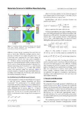
Figure 3. Comparison between modulus and Poisson’s ratio obtained N i =1 ν  ( ) i ( ) i ) ( ν + ˆ ( ) i ˆ ( ) i ) 2  +
2
from finite element simulation and homogenization method:  ( xy − ν xy yx − ν yx  (XVII)
(A) G-Honeycomb and (B) P-Honeycomb.
where N is the number of points in the dataset;
addition, a binary matrix is generated for each lattice to E ()i ,E ()i ν , ()i and ν are the properties predicted by the
i ()
serve as input data. Following topology creation, elastic x y xy yx
modulus and Poisson’s ratio values along both the X- and model; and E ˘ i ,E ˘ i ˘ , and ˘ i are the target properties.
i
Y-directions were computed for each lattice using the x y xy yx
homogenization method. Each data point comprised a
10 × 10 binary matrix representing the lattice topology, An Adam optimizer with a learning rate of 0.001 was
along with corresponding labels: elastic modulus along the used to train the model. A batch size of 64 and 100 epochs
X-direction (E ), elastic modulus along the Y-direction (E ), was set for the training process. Key callbacks, including
y
x
Poisson’s ratio along the X-direction (ν ), and Poisson’s Early Stopping and Model Checkpoint, were integrated to
xy
56
ratio along the Y-direction (ν ). In total, 3000 random enhance training efficiency and prevent overfitting. Input
yx
lattices were generated using this approach. Figure 4 data were reprocessed to improve model performance
presents examples of randomly generated hybrid lattices, before training. Duplicated entries were removed, and
providing visual insight into the diversity and complexity normalization was applied to standardize input features,
of the lattice structures produced. ensuring a well-conditioned dataset with zero mean and
unit standard deviation.
2.6. Architecture of artificial neural network
A back propagation neural network (BPNN) was designed 3. Results and discussion
to train the dataset, utilizing TensorFlow and Keras 3.1. Dataset analysis
frameworks. The architecture of the network unfolds The properties of randomly generated hybrid lattices are
55
sequentially, including an input layer, several hidden layers, analyzed in this section. Figure 6 illustrates the probability
and an output layer, as presented in Figure 5. Commencing density of P-Honeycomb and G-Honeycomb cells across
with a flattening layer to process input 10 × 10 binary the entire dataset. It is evident that both cell types exhibited
matrix, subsequent layers include three densely connected similar probability densities within the dataset, and their
layers with 128, 64, and 32 neurons, respectively. In the distributions can be effectively approximated using a
BPNN, the information from the input layer propagates as normal distribution. The result confirmed the achievement
follows: of a robust randomization process during the generation of
l
Z l A l 1 W l b (XIV) the hybrid lattices.
The mechanical properties of all designs were evaluated
l
l
A f l (XV) using the previously mentioned homogenization method.
Z
Volume 3 Issue 2 (2024) 5 doi: 10.36922/msam.3430