Page 105 - AIH-2-3

Artificial Intelligence in Health Bone suppression utility for chest diagnosis

derive the final labels for the regression models described fold. The training was conducted on an NVIDIA GeForce
in subsection 2.2.3., we averaged the total scores from RTX 4070 with a Windows 11 operating system, utilizing
both radiologists and normalized this value to a floating- Python 3.8.18 and PyTorch 2.2.1.
point number between 0 and 1 by dividing by 18. These Based on our initial experiments, which indicated
normalized scores were used as the labels for the regression that the Stochastic Gradient Descent (SGD) optimizer
models. The mean and standard deviation (SD) of the consistently outperformed the Adam optimizer, we adopted
scores across 192 images were 0.380 and 0.260, respectively. SGD with a learning rate of 0.001 and a momentum of
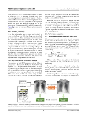
Figure 2 provides an overview of the severity assessment 0.9 for all models. In addition, a learning rate scheduler
process. (StepLR) was applied to reduce the learning rate by a factor
2.2.2. Data pre-processing of 0.1 every 5 epochs.
First, the radiographs were cropped and resized to 2.3. Performance evaluation
center on the lung area, following the process described 2.3.1. Relationship between truths and predictions
in subsection 2.1.2. Next, the images were transformed
into bone-suppressed images using the AI-based bone We compared the performance of the severity assessment
suppression model developed in subsection 2.1. Both the models between the standard chest radiograph dataset
standard radiographs and the bone-suppressed images and the bone-suppressed image dataset by computing the
were independently transformed to a resolution of 512 × mean ± SD of the mean absolute errors (MAEs) and PCCs
512 pixels with 8-bit contrast. Subsequently, each type of across all folds and random seeds. The PCC quantifies the
51
image was then randomly split into training and test data linear relationship between two variables, as expressed by
in an approximately 80:20 ratio, ensuring that all images the following:
i
from the same patient were grouped together in the same n1 x y
y
x
split. Five-fold cross-validation was applied to each dataset r i0 i , (III)
i
i
2
y
separately, and, to enhance robustness, this process was n1 x n1 y 2
x
repeated 3 times using different random seeds. i0 i0
2.2.3. Regression models and training settings Where r is the PCC; x and y denote the individual
i
i
sample points; and x and y are the means of x and y ,
i
i
We employed several CNN architectures from different respectively.
generations – DenseNet, ResNet18, ResNet50, and
47
48
RegNetY-120 – all pre-trained on ImageNet. To adapt These metrics were calculated using the
50
49
these models for the regression task, we modified their final “mean_absolute_error” function from the Python “sklearn.
fully connected layers to have a single output that predicts metrics” library and the “pearsonr” function from the
a continuous value, corresponding to the normalized Python “scipy.stats” module.
Brixia score. These models were trained using the MSE Statistical significance tests were conducted using a
loss function for up to 25 epochs in each cross-validation two-tailed Student’s t-test to compare the average MAEs

Figure 2. Flowchart of coronavirus disease 2019 severity assessment. The Brixia scoring system assigns an integer value from 0 to 3 to each of the six lung
zones (A1 to F1). The total scores from two radiologists were averaged and then normalized to generate the final label scores.

Volume 2 Issue 3 (2025) 99 doi: 10.36922/aih.5608