Page 203 - AJWEP-v22i2

Mitigating climate change in city of Tshwane

decline, loss of business and livelihoods, and increased 3.4. Modeling and simulation of climate change and
investment in repairing damaged infrastructure and mitigation strategies
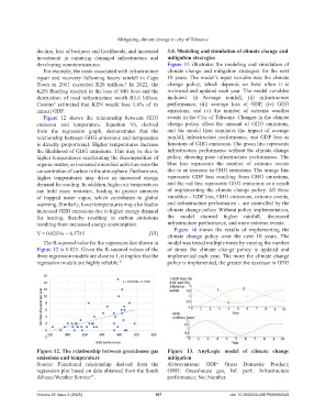
developing countermeasures. Figure 13 illustrates the modeling and simulation of
For example, the costs associated with infrastructure climate change and mitigation strategies for the next
repair and recovery following heavy rainfall in Cape 10 years. The model’s input variable was the climate
Town in 2011 exceeded R20 million. In 2022, the change policy, which depends on how often it is
4
KZN flooding resulted in the loss of 440 lives and the reviewed and updated each year. The model variables
destruction of road infrastructure worth R5.6 billion. included: (i) Average rainfall, (ii) infrastructure
Comins estimated that KZN would lose 1.8% of its performance, (iii) average loss of GDP, (iv) GHG
5
annual GDP. emissions, and (v) the number of extreme weather
Figure 12 shows the relationship between GHG events in the City of Tshwane. Changes in the climate
emission and temperature. Equation VI, derived change policy affect the amount of GHG emissions,
from the regression graph, demonstrates that the and the model then simulates the impact of average
relationship between GHG emissions and temperature rainfall, infrastructure performance, and GDP loss as
is directly proportional. Higher temperatures increase functions of GHG emissions. The green line represents
the likelihood of GHG emissions. This may be due to infrastructure performance without the climate change
higher temperatures accelerating the decomposition of policy, showing poor infrastructure performance. The
organic matter, as increased microbial activities raise the blue line represents the number of extreme events
concentration of carbon in the atmosphere. Furthermore, due to an increase in GHG emissions. The orange line
higher temperatures may drive an increased energy represents GDP loss resulting from GHG emissions,
demand for cooling. In addition, higher air temperatures and the red line represents GHG emissions as a result
can hold more moisture, leading to greater amounts of implementing the climate change policy. All these
of trapped water vapor, which contributes to global variables – GDP loss, GHG emissions, extreme events,
warming. Similarly, lower temperatures may also lead to and infrastructure performance – are controlled by the
increased GHG emissions due to higher energy demand climate change policy. Without policy implementation,
for heating, thereby resulting in carbon emissions the model showed higher rainfall, decreased
resulting from increased energy consumption. infrastructure performance, and more extreme events.
Figure 14 shows the results of implementing the
Y = 0.0254x – 6.5745 (VI) climate change policy over the next 10 years. The

The R-squared value for the regression line shown in model was tested multiple times by varying the number
Figure 12 is 0.825. Given the R-squared values of the of times the climate change policy is updated and
three regression models are close to 1, it implies that the implemented each year. The more the climate change
regression models are highly reliable. 31 policy is implemented, the greater the decrease in GHG

Figure 12. The relationship between greenhouse gas Figure 13. AnyLogic model of climate change
emissions and temperature mitigation
Source: Functional relationship derived from the Abbreviations: GDP: Gross Domestic Product;
regression plot based on data obtained from the South GHG: Greenhouse gas; Inf. perf.: Infrastructure
African Weather Service . performance; No: Number.
37

Volume 22 Issue 2 (2025) 197 doi: 10.36922/AJWEP025080049