Page 198 - AJWEP-v22i2

Sefolo, et al.

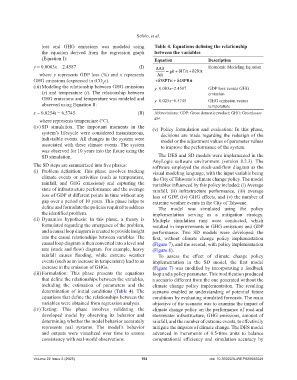
loss and GHG emissions was modeled using Table 4. Equations defining the relationship
the equation derived from the regression graph between the variables
(Equation I): Equation Description
y = 0.0083x − 2.4587 (I) Ait Economic Modeling Equation

where y represents GDP loss (%) and x represents Ait git δ Tit δ1 2 Rit
GHG emissions (expressed in tCO e). δ SPTit δ3 4 SPRit
2
(iii) Modeling the relationship between GHG emissions y=0.083x−2.4587 GDP loss versus GHG
(x) and temperature (t). The relationship between emission
GHG emissions and temperature was modeled and y=0.025x−6.5745 GHG emission versus
observed using Equation II: temperature
x = 0.0254t − 6.5745 (II) Abbreviations: GDP: Gross domestic product; GHG: Greenhouse
where represents temperature (°C). gas.
(iv) SD simulation. The important moments in the (v) Policy formulation and evaluation: In this phase,
system’s lifecycle were considered instantaneous, decisions are made regarding the redesign of the
indivisible events. All changes in the system were model or the adjustment values of parameter values
associated with these climate events. The system to improve the performance of the system.
was observed for 10 years into the future using the
SD simulation. The DES and SD models were implemented in the
The SD steps are summarized into five phases: AnyLogic software environment (version 8.2.3). The
software employed the stock-and-flow diagram as the
(i) Problem definition: This phase involves tracking visual modeling language, with the input variable being
climate events or activities (such as temperature, the City of Tshwane’s climate change policy. The model
rainfall, and GHG emissions) and capturing the variables influenced by this policy included: (i) Average
state of infrastructure performance and the average rainfall, (ii) infrastructure performance, (iii) average
loss of GDP at different points in time without any loss of GDP, (iv) GHG effects, and (v) the number of
gap over a period of 10 years. This phase helps to extreme weather events in the City of Tshwane.
define and formulate the policies required to address The model was simulated using the policy
the identified problem. implementation serving as a mitigation strategy.
(ii) Dynamics hypothesis: In this phase, a theory is Multiple simulation runs were conducted, which
formulated regarding the emergence of the problem, resulted in improvements in GHG emissions and GDP
and a causal loop diagram is created to provide insight performance. Two SD models were developed: the
into the causal relationships between variables. The first, without climate change policy implementation
causal loop diagram is then converted into a level and (Figure 7), and the second, with policy implementation
rate (stock and flow) diagram. For example, heavy (Figure 8).
rainfall causes flooding, while extreme weather To assess the effect of climate change policy
events (such as an increase in temperature) lead to an implementation in the SD model, the first model
increase in the emission of GHGs. (Figure 7) was modified by incorporating a feedback
(iii) Formulation: This phase presents the equations loop and a policy parameter. This modification produced
that define the relationships between the variables, a scenario different from the one generated without the
including the estimation of parameters and the climate change policy implementation. The resulting
determination of initial conditions (Table 4). The scenario enabled an understanding of potential future
equations that define the relationships between the conditions by evaluating simulated forecasts. The main
variables were obtained from regression analysis. objective of the scenario was to examine the impact of
(iv) Testing: This phase involves validating the climate change policy on the performance of road and
developed model by observing its behavior and stormwater infrastructure, GHG emissions, amount of
determining whether the model behavior accurately rainfall, and the number of extreme events, to effectively
represents real systems. The model’s behavior mitigate the impacts of climate change. The DES model
and outputs were visualized over time to ensure advanced in increments of 0.5-time units to balance
consistency with real-world observations. computational efficiency and simulation accuracy by

Volume 22 Issue 2 (2025) 192 doi: 10.36922/AJWEP025080049