Page 128 - AJWEP-v22i3

Fuladipanah, et al.

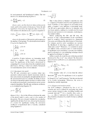
for environmental and hydrological studies. The test n 2
statistic S is calculated using Equation I: t 2 (V)
1
n
n1
S sgn x ( j x ) (I) This t-value follows a Student’s t-distribution with
i
n − 2 degrees of freedom under the null hypothesis of no
i1 ji1
where x and x are the observed values at time points trend. A positive ρ value suggests an increasing trend,
i
j
i and j, and n is the number of data points. Under the null while a negative value indicates a decreasing trend.
hypothesis of no trend, the expected value of S is zero. The SR test is particularly effective for datasets with
The variance of S, denoted as (), is given in Equation II: non-linear patterns, making it a versatile tool for trend
detection and analysis in environmental, hydrological,

VS 1 nn n 5 m t t 2 t 5 and climate studies.
1
12

18 t1 Before conducting the MK and SR tests, the
(II) presence of lag-1 autocorrelation (serial correlation)
where n is the number of data points and m represents must be evaluated. Serial correlation in a dependent
the number of tied groups. The standardized test statistic time series can influence the effectiveness of these tests.
Z is given by Equation III: For instance, positive serial correlation can increase
the likelihood of detecting a significant trend even
S 1 40
; if S 0 when none exists. Therefore, it is essential to assess
VS () and address serial correlation prior to trend analysis.

Z 0; S 0 (III) If significant serial correlation is present, test statistics
S 1 must be adjusted, or a pre-whitening technique should
; if S 0 be applied to eliminate its impact.
VS () In this research, the trend-free pre-whitening method

41
A positive Z-value indicates an increasing trend, introduced by Yue et al. was utilized. The first-order
whereas a negative value signifies a decreasing autocorrelation coefficient (r ) is calculated as shown in
i
trend. The significance of the trend is determined by Equation VI:
comparing Z to critical values from the standard normal 1 Ni
distribution, offering a robust and reliable framework Ni k1 ( x x x)( i k x)

i
for trend detection across diverse datasets. r 1 N 2 (VI)
i
x
k
N k1 ( x )
2.2.2. Spearman’s rho model
The SR rank correlation test is another robust non- If the absolute value of r is less than the critical
1
parametric method used to identify monotonic trends in threshold 196. at the 5% significance level, as applied
time series data by measuring the strength and direction of N
43
42
the association between two variables. Its ability to detect by Douglas et al. and Tosunoglu, the data are deemed
non-linear relationships and its resistance to outliers make to be serially independent. Otherwise, the series is
it a widely used approach in trend analysis across various classified as serially dependent.
scientific disciplines. The SR rank correlation coefficient,
ρ, is calculated using Equation IV: 2.2.3. Polygon trend analysis model
The IPTA technique, introduced by Sen et al., is
7
n
6 d i 2 versatile and can be utilized for analyzing time series
1 i 1 (IV) across various temporal scales, including monthly and
nn ( 2 1)
seasonal intervals. 44-48 For a monthly time series x ,
1
where d =R(x ) − R(y ) is the difference between the ranks x ,…, x , where n represents the number of years, the
2
n
i
i
i
of the paired values x and y , and n is the number of data should be structured in a matrix format as outlined
i
i
7
data points. The test evaluates whether the calculated ρ by Sen et al. :
significantly deviates from zero, indicating the presence x 11, x 12 1,
of a trend. For significance testing, the correlation
coefficient is transformed into a t-statistic, calculated x
using Equation V. 1, n x 12, n
Volume 22 Issue 3 (2025) 122 doi: 10.36922/AJWEP025080052