Page 90 - IJAMD-1-2

International Journal of AI for
Materials and Design
AMTransformer for process dynamics

5.1. Data selection and laser velocity and energy per unit length (mm) as

To assess the learning capabilities of the AMTransformer, rate properties of the laser to understand their dynamical
we utilized the AM metrology testbed (AMMT): dependencies and predict future melt pools. To extract
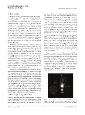
overhang part X4 dataset, which was created to facilitate features from the raw data, we performed three types
the development of data-driven predictive models, as of pre-processing on the raw MPM images: denoising,
centering, and cropping, in addition to pre-processing
referenced in Lane and Yeung. This dataset was compiled the control data. These datasets encompass a variety of
39
through research conducted at the National Institute dynamic AM phenomena, including but not limited to
of Standards and Technology. The AMMT building melt pools, spatter, and plumes, as shown in Figure 7. The
process involves constructing four overhang structures extracted features of these phenomena serve as critical
measuring 5 mm × 9 mm × 5 mm. The process involves indicators for understanding and categorizing the state and
a laser with a specified power of 100 W and a scanning rate properties within the LPBF process.
speed of 900 mm/s for the pre-contour phase. During
the infill hatching phase, the laser power is increased to The denoising process removed any noise from the raw
195 W, and the scanning speed is adjusted to 800 mm/s. MPM images, such as the noise highlighted in Figure 7,
The component is fabricated by accumulating 250 layers, leaving only the features of interest: the main melt pool,
each with a thickness of 20 μm, with a 90° rotation applied spatter, and plume. After denoising, we centered and
between each layer. cropped the main melt pools. Centering reduced bias
related to the locations of the melt pools in the images,
The AMMT dataset encompasses a collection of in situ while cropping decreased the size of the original MPM
MPM images captured during the execution of an LPBF images from 120 × 120 pixels to 64 × 64 pixels for enhanced
process, as well as a set of process control commands and resource utilization. Figure 8 illustrates the pre-processing
measured data. The MPM images are captured using a of the MPM images.
co-axial MPM camera integrated into the AMMT. To obtain
stationary monitoring images of the melt pool during the We also processed the control data to extract additional
3D build process, the laser beam and melt pool emission features such as laser velocity and energy per unit length.
are optically aligned in the system, ensuring that the high- For laser velocity, we measured the times and the distances
speed camera’s field of view is fixed on the melt pool. The traveled by the laser. Distances were measured based on
camera captures 120 × 120-pixel grayscale images of melt the x and y coordinates using the Pythagorean theorem.
pools at a sampling rate of 100 μs per frame, with pixel We then extracted the laser velocity feature by dividing the
values ranging from 0 to 255. The command data for the distance by the time, according to the formula for velocity
process contains information regarding the location and in physics. Using the laser’s velocity and power, we also
power required for controlling the laser. 39 extracted the feature for the energy per unit length – a
measure of how much energy is applied per unit length –
In this study, we employed a total of 13,233 MPM images, by dividing the power by the velocity.
specifically from the fourth part of the dataset. We selected
4812 images from Layer 1, 3609 images from Layer 150,
and another 4812 images from Layer 210, along with the
corresponding process control information. These layers were
chosen because they exhibited a high incidence of anomalies,
thereby providing a comprehensive dataset for our model
analysis. To ensure the reliability of our results, we set aside
18% (2406 images) of the total dataset as the test dataset.
This selection was done randomly across the different layers
(Layer 1, Layer 150, and Layer 210) to ensure a representative
sample. The test dataset was used to evaluate the model’s
performance and validate its accuracy. The remaining 82%
(10,827 images) of the data was used for training.
5.2. Data pre-processing and structure

The AMTransformer used the pre-processed MPM images
representing the melt pool, spatter, and plume areas, along Figure 7. An example of a melt pool monitoring (MPM) image: the
with the melt pool’s x and y locations as state properties orange circle highlights a noise instance, displaying random greyscale
of the material, laser power as state property of the laser, variations in the MPM images outside the melt pool, spatter, and plume

Volume 1 Issue 2 (2024) 84 doi: 10.36922/ijamd.3919