Page 92 - IJAMD-1-2

International Journal of AI for
Materials and Design
AMTransformer for process dynamics

gradient problem. 40,41 In this case study, we trained the image x and the predicted image y – based on luminance,
AM state embedder for 300 epochs, after which the contrast, and structure. We calculated each comparison
43
trained embeddings were passed to the transformer. As a factor using Equation XV. Utilizing the results from this
sequence of AM state embeddings from the LPBF process equation, we derived the SSIM using Equation XVI, where
is processed through the transformer, the proposed model µ and σ represent the average and variance, respectively,
identifies non-local dynamic dependencies in LPBF using and c denotes a constant.
the attention mechanism and infers future states based on 2 c 2 c
its understanding, as shown in Figure 9C. The transformer lx y, x y 1 , cx y , x y 2 ,
consists of six decoder layers, with each decoder having x 2 2 y c 1 x 2 y 2 c 2
four heads of attention. The feed-forward neural networks xy c 3
in the transformer adopted the GELU activation function, sx y , c (XV)
which offers smoother and more probabilistic activation, x y 3
potentially enhancing the model’s performance. The SSIM xy, lx yc xy sx y, , ,
42
length of each AM state embedding sequence input for the
transformer was set to 16, and the transformer was trained (2 y c )(2 xy c ) (XVI)
x
2
1
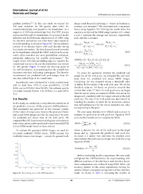
for 200 epochs. Figure 10 shows the learning curve of ( 2 c )( 2 2 c )
2
the AMTransformer, demonstrating how the model’s loss x y 1 x y 2
decreases over time, indicating convergence. The decoder To assess the agreement between the predicted and
reconstructed the predicted melt pool images from the actual size of the melt pools, we extracted the melt pool
outcome embeddings of the transformer. areas from the predicted and actual MPM images.
Experiments were conducted in a Linux environment Calculating the size required setting a threshold value
with an Intel Xeon CPU (2 cores @2.00GHz), 12.7GB to define the boundary of the melt pool area. We set the
RAM, and an NVIDIA Tesla T4 GPU. The software used in threshold value to 150 based on previous research that
this study included Python 3.10, PyTorch 2.3, and CUDA verified this value. 15,23 Since the melt pool areas are larger
12.2. than the spatter areas, we examined all the contours in the
images and considered only the largest contour as the melt
5.4. Results pool area. The size of the melt pools was determined by
counting the number of pixels in the maximum contour
In this study, we conducted a comprehensive evaluation of area and multiplying it by the actual measured size value
the predictive accuracy of the proposed AMTransformer. corresponding to the pixel.
This assessment was grounded in two primary criteria:
(i) the extent of congruence between the predicted future We used mean absolute error (MAE) and accuracy to
and actual MPM images and (ii) the congruence between evaluate the prediction of melt pool size. Equation XVII
the predicted and actual sizes of the melt pools. We presents the formula used to compute the MAE:
compared the AMTransformer model against a transformer 1
with a basic autoencoder model and a convolutional LSTM MAE = ∑ i n =1 α i α − ˆ i (XVII)
(ConvLSTM) model based on these criteria. n
To evaluate the generated MPM images, we used the where α denotes the size of the melt pool in the target
i
structural similarity (SSIM) metric. SSIM assesses this image and α ˆ represents the predicted melt pool size.
i
similarity between two images – namely, the ground truth Accuracy is a metric that calculates the absolute error
ratio between the predicted and target melt pool size using
Equation XVIII:
α α − ˆ
Accuracy i = −1 i α i i (XVIII)

Before conducting model comparisons, the case study
configured the AMTransformer by experimenting with
different numbers of decoder layers and attention heads.
Each configuration was evaluated using SSIM, MAE, and
accuracy metrics. In the initial experiments varying the
number of layers, we used a configuration of four attention
Figure 10. The learning curve of the AMTransformer heads. As shown in Table 1, increasing the number of

Volume 1 Issue 2 (2024) 86 doi: 10.36922/ijamd.3919