Page 200 - IJOCTA-15-1

H.H. Yildirim, A. Akusta / IJOCTA, Vol.15, No.1, pp.183-201 (2025)
Table 4. Variables and acronyms
used in the research

Acronyms Variables Variable Type
vol Volatility Dependent Variable
co Current Ratio
bo Leverage Ratio ( Borrowing Ratio)
adh Asset Turnover Ratio
roa Return on Assets Independent Variable
roe Return on Equity
pddd Market Value / Book Value
beta Firm Beta
Sources: Authors’ Finding.

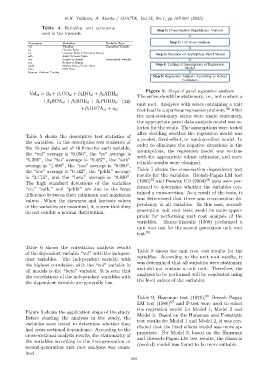
Figure 3. Steps of panel regression analysis
Vol it = β 0 + β 1 CO it + β 2 BO it + β 3 ADH it
The series should be stationary, i.e., not contain a
+β 4 ROA it + β 5 ROE it + β 6 PDDD it (34)
unit root. Analyses with series containing a unit
+β 7 BETA it + u it 56
root lead to a spurious regression problem. After
the non-stationary series were made stationary,
the appropriate panel data analysis model was se-
lected for the study. The assumptions were tested
after deciding whether the regression model was
Table 5 shows the descriptive test statistics of
a pooled, fixed-effect, or random-effect model. In
the variables. In the descriptive test statistics of
order to eliminate the negative situations in the
the 18-year data set of 46 firms for each variable,
assumptions, the regression model was re-done
the “vol” average is “0.056”, the “co” average is
with the appropriate robust estimator, and more
“5.396”, the “bo” average is “0.487”, the “adh”
reliable results were obtained.
average is “1.090”, the “roa” average is “0.080”,
Table 7 shows the cross-section dependency test
the “roe” average is “0.142”, the “pddd” average
results for the variables. Breush-Pagan LM test
is “3.173”, and the “beta” average is “0.830”. 57 58
(1980) and Pesaran CD (2004) tests were per-
The high standard deviations of the variables
formed to determine whether the variables con-
“co,” “adh,” and “pddd” are due to the large
tained a cross-section. As a result of the tests, it
difference between their minimum and maximum
was determined that there was cross-section de-
values. When the skewness and kurtosis values
pendency in all variables. In this case, second-
of the variables are examined, it is seen that they
do not exhibit a normal distribution. generation unit root tests would be more appro-
priate for performing unit root analysis of the
variables. Harris-Tzavalis (1999) performed a
unit root test for the second generation unit root
test. 59
Table 6 shows the correlation analysis results
Table 8 shows the unit root test results for the
of the dependent variable “vol” with the indepen-
variables. According to the unit root results, it
dent variables. The independent variable with
was determined that all variables were stationary
the highest correlation with the “vol” variable in
and did not contain a unit root. Therefore, the
all models is the “beta” variable. It is seen that
analyses to be performed will be conducted using
the correlations of the independent variables with
the level values of the variables.
the dependent variable are generally low.
Table 9, Hausman test (1978), 60 Breush Pagan
LM test (1980) 57 and F-test were used to select
the regression model for Model 1, Model 2 and
Figure 3 shows the application steps of the study.
Model 3. Based on the Hausman and F-statistic
Before starting the analysis in the study, the
test results for Model 1 and Model 2, it was con-
variables were tested to determine whether they
cluded that the fixed effects model was more ap-
had cross-sectional dependence. According to the
propriate. For Model 3, based on the Hausman
cross-sectional analysis results, the stationarity of
and Breusch-Pagan LM test results, the classical
the variables according to the first-generation or
(pooled) model was found to be more suitable.
second-generation unit root analyses was exam-
ined.
194