Page 49 - IJOCTA-15-1

Approximate analytical solutions of fractional coupled Whitham-Broer-Kaup equations . . .

0.4 0.4
0.2 0.2
0 0
−0.2 −0.2
−0.4 −0.4
1 1
−100 −100
0.8 0.8
−50 −50
0.6 0.6
0 0
0.4 0.4
50 0.2 50 0.2
0
0
100 100
(a) (b)
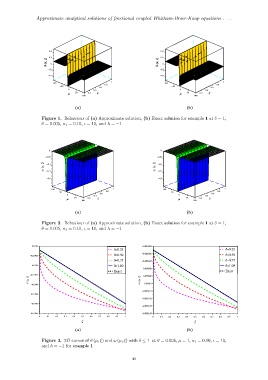
Figure 1. Behaviour of (a) Approximate solution, (b) Exact solution for example 1 at δ = 1,
θ = 0.005, κ 1 = 0.10, ι = 10, and ℏ = −1

0 0
−0.05 −0.05
−0.1 −0.1
−0.15 −0.15
−0.2 −0.2

−100 1 −100 1
0.8 0.8
−50 −50
0.6 0.6
0 0
0.4 0.4
50 0.2 50 0.2
1000 1000
(a) (b)
Figure 2. Behaviour of (a) Approximate solution, (b) Exact solution for example 1 at δ = 1,
θ = 0.005, κ 1 = 0.10, ι = 10, and ℏ = −1

−0.11992 −0.005605
ð=0.25
ð=0.25 ð=0.25
ð=0.25ð=0.25
ð=0.25
ð=0.25
ð=0.25
ð=0.25ð=0.25
ð=0.50 −0.005606 ð=0.50
ð=0.50
ð=0.50
ð=0.50ð=0.50
ð=0.50
ð=0.50
ð=0.50ð=0.50
−0.119925
ð=0.75 −0.005607 ð=0.75
ð=0.75
ð=0.75ð=0.75
ð=0.75
ð=0.75
ð=0.75
ð=0.75ð=0.75
ð=1.00
ð=1.00
ð=1.00
ð=1.00ð=1.00
ð=1.00
ð=1.00ð=1.00
−0.11993 ð=1.00 ð=1.00
−0.005608
ExactExact
Exact
Exact
Exact
Exact
Exact Exact
ExactExact
−0.119935
−0.005609
−0.00561
−0.11994
−0.005611
−0.119945
−0.005612
−0.11995
−0.005613
−0.119955 −0.005614
0 0.1 0.2 0.3 0.4 0.5 0.6 0.7 0.8 0.9 1 0 0.1 0.2 0.3 0.4 0.5 0.6 0.7 0.8 0.9 1
(a) (b)
Figure 3. 2D curves of ϑ (µ, ξ) and ω (µ, ξ) with δ ≤ 1 at θ = 0.005, µ = 1, κ 1 = 0.10, ι = 10,
and ℏ = −1 for example 1
43