Page 51 - IJOCTA-15-1

Approximate analytical solutions of fractional coupled Whitham-Broer-Kaup equations . . .

−0.24484 −0.01121
ð=0.25
ð=0.25ð=0.25
ð=0.25
ð=0.25ð=0.25ð=0.25ð=0.25
ð=0.25 ð=0.25
ð=0.50
ð=0.50 ð=0.50
ð=0.50
ð=0.50ð=0.50ð=0.50ð=0.50
ð=0.50ð=0.50
−0.24485 −0.011215
ð=0.75 ð=0.75
ð=0.75
ð=0.75
ð=0.75ð=0.75
ð=0.75ð=0.75ð=0.75ð=0.75
ð=1.00
ð=1.00
ð=1.00ð=1.00ð=1.00ð=1.00
−0.24486 ð=1.00 −0.01122 ð=1.00
ð=1.00ð=1.00
Exact
Exact Exact
Exact
ExactExact
ExactExactExactExact
−0.24487 −0.011225
−0.24488 −0.01123
−0.24489 −0.011235
−0.2449 −0.01124
−0.24491 −0.011245
0 0.1 0.2 0.3 0.4 0.5 0.6 0.7 0.8 0.9 1 0 0.1 0.2 0.3 0.4 0.5 0.6 0.7 0.8 0.9 1
(a) (b)
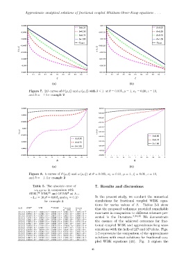
Figure 7. 2D curves of ϑ (µ, ξ) and ω (µ, ξ) with δ ≤ 1 at θ = 0.005, µ = 1, κ 1 = 0.10, ι = 10,
and ℏ = −1 for example 2
−0.244844 −0.011211
−0.011212
−0.244846
−0.011213
−0.244848
−0.011214
−0.011215
−0.24485
−0.011216
−0.244852 ð=0.50
ð=0.50ð=0.50
−0.011217
ð=0.50
ð=0.50ð=0.50 ð=0.75
ð=0.75ð=0.75
−0.011218
−0.244854
ð=0.75
ð=0.75ð=0.75
ð=1.00
ð=1.00ð=1.00
ð=1.00ð=1.00
ð=1.00 −0.011219
−0.244856
−0.01122
−0.244858 −0.011221
−2 −1.8 −1.6 −1.4 −1.2 −1 −0.8 −0.6 −0.4 −0.2 0 −2 −1.8 −1.6 −1.4 −1.2 −1 −0.8 −0.6 −0.4 −0.2 0
(a) (b)
Figure 8. ℏ curves of ϑ (µ, ξ) and ω (µ, ξ) at θ = 0.005, κ 1 = 0.10, µ = 1 , ξ = 0.01 , ι = 10,
and ℏ = −1. for example 2
Table 5. The absolute error of 7. Results and discussions
ω HAST M in comparison with
4
ADM, 34 VIM, 35 and OHAM at ℏ =
−1, ι = 10, θ = 0.005, and κ 1 = 0.10 In the present study, we conduct the numerical
for example 2. simulations for fractional coupled WBK equa-
tions for varies values of δ. Tables 2-5 show
(µ, ξ) ADM 34 V IM 30 OHAM 4 ω HASTM ω HASTM that the proposed technique provided remarkable
(δ = 0.75) (δ = 1)
(0.1, 0.1) 6.41419 × 10 −3 1.10430 × 10 −4 5.86860 × 10 −5 3.3080 × 10 −5 1.3878 × 10 −17
(0.1, 0.3) 5.99783 × 10 −3 3.31865 × 10 −4 3.04565 × 10 −4 4.7354 × 10 −5 3.4694 × 10 −16 exactness in comparison to different schemes pre-
(0.1, 0.5) 5.61507 × 10 −3 5.54071 × 10 −4 3.08812 × 10 −4 5.0855 × 10 −5 2.4009 × 10 −15 4,34,35
(0.2, 0.1) 1.33181 × 10 −2 1.07016 × 10 −4 5.56884 × 10 −5 3.2058 × 10 −5 6.9389 × 10 −17 sented in the literature. We demonstrate
(0.2, 0.3) 1.24441 × 10 −2 3.21601 × 10 −4 2.97260 × 10 −4 4.5890 × 10 −5 3.1919 × 10 −16
(0.2, 0.5) 1.16416 × 10 −2 5.36927 × 10 −4 2.92626 × 10 −4 4.9283 × 10 −5 2.3176 × 10 −15 the essence of the achieved outcomes for frac-
(0.3, 0.1) 2.07641 × 10 −2 1.03737 × 10 −4 5.28609 × 10 −5 3.1075 × 10 −5 4.1633 × 10 −17
(0.3, 0.3) 1.93852 × 10 −2 3.11737 × 10 −4 2.90510 × 10 −4 4.44836 × 10 −5 2.6368 × 10 −16 tional coupled WBK and approximate long wave
(0.3, 0.5) 1.81209 × 10 −2 5.20447 × 10 −4 2.77382 × 10 −4 4.7771 × 10 −5 2.1233 × 10 −15
(0.4, 0.1) 2.88100 × 10 −2 1.00579 × 10 −4 5.01929 × 10 −5 3.0129 × 10 −5 2.7756 × 10 −17 equations with the help of 2D and 3D plots. Figs.
(0.4, 0.3) 2.68724 × 10 −2 3.02245 × 10 −4 2.83229 × 10 −4 4.3129 × 10 −5 2.3592 × 10 −16
(0.4, 0.5) 2.50985 × 10 −2 5.04593 × 10 −4 2.63019 × 10 −4 4.6316 × 10 −5 2.0410 × 10 −15 1-2 represents the comparison of the approximate
(0.5, 0.1) 3.75193 × 10 −2 9.75385 × 10 −5 4.76741 × 10 −5 2.9219 × 10 −5 1.3878 × 10 −17
(0.5, 0.3) 3.49617 × 10 −2 2.93107 × 10 −4 2.76492 × 10 −4 4.1826 × 10 −5 2.6368 × 10 −16 solutions with exact solutions for fractional cou-
(0.5, 0.5) 3.26239 × 10 −2 4.89335 × 10 −4 2.49480 × 10 −4 4.4917 × 10 −5 1.9013 × 10 −15
pled WBK equations (41). Fig. 3 explore the
45