Page 104 - IJOCTA-15-2

Collocation method with flood-based metaheuristic optimizer for optimal control ...

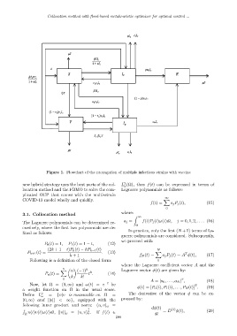
Figure 1. Flowchart of the propagation of multiple infectious strains with vaccine

2
new hybrid strategy uses the best parts of the col- L (Ω), then f(t) can be expressed in terms of
ω
location method and the FBMO to solve the com- Laguerre polynomials as follows:
plicated OCP that comes with the multi-strain
∞
COVID-19 model wholly and quickly. X
f(t) = a j P j (t), (15)
0
where:
3.1. Collocation method
Z ∞
The Laguerre polynomials can be determined re- a j = f(t)P j (t)ω(t)dt, j = 0, 1, 2, . . . . (16)
0
cursively, where the first two polynomials are de-
fined as follows: In practice, only the first (N +1) terms of La-
guerre polynomials are considered. Subsequently,
we proceed with:
P 0 (t) = 1, P 1 (t) = 1 − t, (12)
(2k + 1 − t)P k (t) − kP k−1 (t) N
P k+1 (t) = . (13) X T
k + 1 f N (t) = a j P j (t) = A ϕ(t), (17)
Following is a definition of the closed form: 0
where the Laguerre coefficient vector A and the
n k
X n (−1) k Laguerre vector ϕ(t) are given by:
P n (t) = t . (14)
k k!
0 A = [a 0 , . . . , a N ] , (18)
T
Now, let Ω = (0, ∞) and ω(t) = e −t be T
a weight function on Ω in the usual sense. ϕ(t) = [P 0 (t), P 1 (t), . . . , P N (t)] . (19)
Define L 2 ω = {v|v is measurable on Ω = The derivative of the vector ϕ can be ex-
(0, ∞) and ||v|| < ∞}, equipped with the pressed by:
following inner product and norm: (u, v) ω =
1 dϕ(t) (1)
R 2 = D ϕ(t), (20)
u(t)v(t)ω(t)dt, ||v|| ω = (u, v) ω . If f(t) ∈
Ω dt
299