Page 108 - IJOCTA-15-2

Collocation method with flood-based metaheuristic optimizer for optimal control ...
Initialize the sizes of the control parameters of the FBMO,
i.e., the scaling element Ne, the maximum number of repetitions (Iter_{max}),
the mass size (N_{pop}),
and the repetition number (Iter=0) for the crowd.
1: To generate the randomly initial swarm N_{pop} (i=1,...,N_{pop});
2: U_{i}=U_{min}+rand*(U_{max}-U_{min})
3: To compute the objective functional of the initial random mass;
4: While the i till Iter_{max}, do
5: To arrange the repetitions, Iter=Iter+1;
6: for i=1 to N_{pop}, do
7: Pe_{i}=(J(U_{i})-J_{min}/J_{max}-J_{min})^2
8: if randG>rand+Pe_{i} then
9: U_{i}^{new}=U_{i}+(Pk^{rand}/Iter)*(rand*(U_{max}-U_{min})+U_{min})
10: else
11: U_{i}^{new}=U_{best}+rand*(U_{j}-U_{i})
12: end if
13: if J(U_{i}^{new})<J(U_{i}) then
14: U_{i}=U_{i}^{new} and J(U_{best})=J(U_{i});
15: end if
16: if J(U_{i})<J(U_{best}) then
17: U_{best}=U_{i} and J(U_{best})=J(U_{i});
18: end if
19: end for
20: if rand<Pt ; Pt=|sin(rand/Iter)| then
21: for e=1 to Ne, do
22: U_{e}^{new}=U_{best}+rand*(rand*(U_{max}-U_{min})+U_{min})
23: if J(U_{e}^{new}) < J(U_{best})
24: U_{best}=U_{e}^{new} and J(U_{best})=J(U_{e}^{new});
25: end if
26: end for
27: end if
28: end while
Output: U_{best}

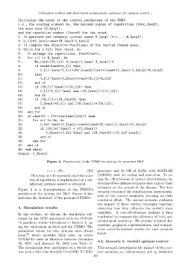
Figure 2. Pseudo-code of the FBMO for solving the presented NLP

e = 1 : Ne. (59) processor and 16 GB of RAM, with MATLAB
This step will be repeated until the num- (R2023b) used for coding and execution. To as-
ber of repetitions is implemented or a sat- sess the effectiveness of control interventions, we
isfactory optimal answer is obtained. developed two distinct scenarios that explore their
influence on the spread of the disease. The first
Figure 2 is a demonstration of the FBMO’s
scenario examines the simultaneous implementa-
pseudo-code for solving the NLP. Figure 3 also
tion of two control measures, focusing on their
indicates the flowchart of the presented FBMO.
combined effect. The second scenario evaluates
the impact of three control strategies together,
4. Simulation results observing how they influence the model’s state
variables. A cost-effectiveness analysis is then
In this section, we discuss the simulation out-
comes for the OCP associated with the COVID- conducted to compare the efficiency of both epi-
19 pandemic model introduced in Section 2, us- demiological scenarios. We provide detailed dis-
ing the collocation method and the FBMO. The cussions, graphical representations, and compar-
ative cost-effectiveness results for each scenario
parameter values for this analysis were drawn
from, 20 which provides daily data on active below.
COVID-19 cases in Morocco between December
4.1. Scenario 1: twofold optimal control
28, 2021, and January 16, 2022 (see Table 4).
The simulations were performed on a 64-bit sys- This scenario investigates the impact of two con-
tem with a 12th Gen Intel(R) Core(TM) i7-1255U trol variables, u 1 (vaccination) and u 2 (isolation
303