Page 39 - IJOCTA-15-3

Modeling and analysis of the dynamics of an excessive gambling problem with modified fractional operator
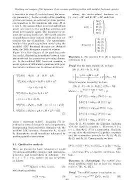
a transition to stage R, modeled using the recov- where, the vector-valued functions m :
5
5
5
ery parameter ζ. As the severity of the gambling [0, +∞) → R and Φ : R → R such that
problem decreases, an addicted problem gambler  
N (t)
can transition to the minimum risk stage M at
 A (t) 
a rate δ. We assumed that recovered individuals  
m (t) =  M (t)  ,
would not return to the gambling activities and  
P (t)
 
would never gamble again. The parameter ψ de-
R (t)
notes the natural death rate. The model assumes
and
no gambling problem-induced death and does not  
Φ 1 (t)
consider the age of gamblers. The approximate
 Φ 2 (t) 
results of the gambling problem model using the  
Φ (m (t)) =  Φ 3 (t)  .
modified ABC fractional operator are obtained  
 Φ 4 (t) 
using the Tofik-Atangana numerical scheme.
Φ 5 (t)
Figure 1 is a flow diagram of the gambling prob-
lem model, illustrating transitions between com-
Theorem 1. The function Φ in (8) is Lipschitz
partments and key parameters governing dynam-
continuous in η.
ics. In the modified ABC fractional operator, a
model system of differential equations with posi-
tive initial conditions can be defined as follows: Proof. For the state variable N, we have
∥Φ 1 (t, N) − Φ 1 (t, N 1 )∥
D N(t) = Φ 1 (t) = Λ − ϑ 1 N − ψN,
 ∗ υ
γ 1 A + γ 2 M + γ 3 P
 t = α 1 + ψ ∥N 1 − N∥ .



T


 ∗ υ
 D A(t) = Φ 2 (t) = ϑ 1 N + λM + κP
 t Using triangular inequality, we have




 ∥Φ 1 (t, N) − Φ 1 (t, N 1 )∥ ≤ c ∥N 1 − N∥ .
− (℘ + ϑ 2 + ψ) A,




γ 1 ϱ 2 + γ 2 ϱ 3 + γ 3 ϱ 3


 where c = α 1 + ψ.
∗ D M(t) = Φ 3 (t) = ϑ 2 A + δP . T
υ
t


  ∥N (t) ∥ = sup |N (t) | = ϱ 1 ,
 t∈T
 
 − (λ + ς + ϑ 3 + ψ) M, 




 
 
  ∥A (t) ∥ = sup |A (t) | = ϱ 2 ,

 t∈T
 ∗ υ 

 D P(t) = Φ 4 (t) = ϑ 3 M − (κ + δ + ζ + ψ)P, 


t
 

 ∥M (t) ∥ = sup |M (t) | = ϱ 3 ,
 t∈T
υ
∗ D R(t) = Φ 5 (t) = ℘A + ςM + ζP − ψR. 

t



(7)  ∥P (t) ∥ = sup t∈T |P (t) | = ϱ 4 ,







∥R (t) ∥ = sup t∈T |R (t) | = ϱ 5 .

where ∗ represents mABC. Equation (7) de-
Thus, Φ 1 (t, N) satisfies the Lipschitz condition
scribes the rates of change for each compartment,
incorporating fractional-order dynamics via the with the Lipschitz constant c. Moreover, if 0 ≤
c < 1, then Φ 1 (t, N) is a contraction. Similarly,
modified ABC operator. Parameters ϑ 1 , ϑ 2 and
we can show the existence of Lipschitz constants
ϑ 3 demonstrate model transitions influenced by
and the contraction principle for Φ 2 (t), Φ 3 (t),
problem gambler interactions.
Φ 4 (t), and Φ 5 (t). Consequently, we have:
3.1. Qualitative analysis
∥Φ (t, m (t)) − Φ (t, m 1 (t)) ∥ ∞ ≤ η Φ ∥m − m 1 ∥ ∞ .
Here, we discuss the basic behaviors of model (10)
(7) such as solvability, existence and uniqueness, and hence Φ is a Lipschitz continuous func-
positivity, and boundedness of solutions. For tion.
0 < t < T < +∞, system (7) can be written
as follows: Theorem 2. (Solvability) The mABC frac-
tional gambling model has at least one solution
mABC υ 5
D m (t) = Φ (t, m (t)) , (8) m(t) ∈ C [0, τ] , R + .
0
with starting solution
Proof. The mABC system is equivalent to:
υ
m (0) = m 0 , (9) m (t) − m 0 = mAB I Φ (t, m (t)) . (11)
0
411