Page 227 - IJOCTA-15-4

Data-driven optimization and parameter estimation for an epidemic model
Appendix A. Data pre-processing methodology has been employed in many other
epidemic modeling studies. 53,58–61
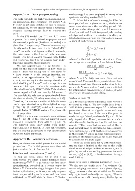
The daily raw data are highly oscillatory, indicat-
To follow Schmitt’s methodology, let P be the
ing inconsistent daily reporting - see Figure A11.
total population at a given vertex v, which we as-
In order to get data suitable for use in parame- sume is constant over the modeling period. We
ter estimation, we pre-process using a Gaussian-
weighted moving average filter to smooth the work over a short time period on which we assume
data. S ≈ P, α = 0, and λ = 0, temporarily decoupling
all edges and vertices. On this short timeline, the
In the SIR model, the I(t) and R(t) terms
represent the currently infectious population and infected population I and the removed population
the removed population (deaths + recoveries) at a R grow at each vertex as follows:
given time t, respectively. These values are rarely
directly available from data. For the Poland MOH d I = (βP − η) I
data, 64 as with most typical epidemic datasets, dt
the data come in the form of daily new case d R = ηI,
counts. The MOH dataset contains both deaths dt
and recoveries, but it is not obvious how under- where P is the total population at vertex v. Thus,
reporting impacted these numbers. we can approximate β and η from data as follows:
We can approximate I(t) as follows: let R(t + 1) − R(t)
N(t) be the reported number of new cases at ∆t ≈ ηI(t)
time t. Then the rolling sum of new cases for I(t + 1) − I(t)
n days, where n is the average infection du- ∆t ≈ (βP − η) I(t),
ration, is an approximation for I(t). We let where ∆t = 1 for daily case data. Note that val-
n = 6, accounting for the average duration of ues of I and R are not directly available and have
viral shedding of 5 days 48 and average time to to be computed from the data as described in Ap-
death of 14.8 days, 111 which is consistent with pendix A. At each vertex, β and η are multiplied
other studies of early COVID-19 in Poland where by optimization parameters c β (v) and c η (v) to be
deaths lagged behind new cases by 2-3 weeks. 112 determined through model fitting.
The case fatality rate can be approximated from
the data as deaths/(deaths+recoveries) ≈ 2.6%. Vertex to edge (λ)
v
Therefore, the average duration of infectiousness λ is the rate at which individuals leave vertex v
e
can be approximated using the weighted average to travel on edge e. We use traffic data from a
(0.026)(14)+(1−0.026)(5) ≈ 5.6, which we round 2022 Polish government report 113 to inform this
up to 6. Later COVID-19 variants likely have dif- parameter. Most of the edges in our network may
ferent properties. be classified in terms of the main European E-
R(t) is the cumulative removed population at roads through Poland, as shown in Figure 1. If the
time t. Let M be the reported removed cases edge is part of an E-road, we associate a number
P τ=t
(deaths + recoveries). Then R(t) ≈ M(τ). with the traffic density on that E-road from the
τ=0
The removed cases likely suffer from under- report. 113 The roads that are not part of the E-
reporting, as it is difficult to track all recoveries, road network may be classified by type (express-
but the scaling parameters in our optimization way, highway, etc.), with traffic density also given
adjust for under-reporting. in the report. 113 When an edge represents multi-
ple routes, the traffic densities are added together
Appendix B. Parameter selection to account for multiple edges.
v
Here, we discuss our initial guesses for the model Then the initial guess for λ is the traffic den-
e
parameters. The initial guesses were then ad- sity on edge e divided by the sum of the traffic
justed as described in Section 2.3. densities on all edges incident to vertex v, multi-
plied by an unknown scaling parameter for each
Infection and removal rates (β and η)
vertex, c λ (v) ∈ (0, 1), to be determined through
To find an initial guess for β and η at model fitting.
each vertex, we adapt a finite-difference-based
methodology, 53,58–61 in particular the first-order Edge m to edge n skipping parameter (v e m ,e n )
approximation described in a recent paper by We also use the traffic data 113 to estimate the
Schmitt. 59 This methodology, is a good first guess vertex skipping parameter. For a given edge e m ,
before optimization, as it requires only approx- v v represents the rate at which traffic leaves
e m,e n
imate exponential growth rates and has been edge e m to travel to the adjacent edge e n . We esti-
validated on COVID data in France. 59 Similar mate it as the traffic density on e n divided by the
769