Page 228 - IJOCTA-15-4

H. Kravitz et al. / IJOCTA, Vol.15, No.4, pp.750-778 (2025)

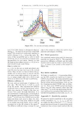
Figure A11. The raw data are highly oscillatory.

sum of the traffic density on all adjacent edges ex- edge in the network to reduce the number of pa-
cluding e m . As noted in our previous coupled 2D rameters and mitigate overfitting.
study, 30 the model is not particularly sensitive to
uniform changes in v v across edge pairs. Be- B.1. Model parameters
e m,e n
cause of this insensitivity and in order to avoid
The populated vertices along with the vertex pa-
overfitting, we do not introduce a separate scal-
rameters are found in Table 3. The edge-based
ing parameter for each vertex. Instead, we find
parameters (diffusion coefficients and the traffic
the single global scaling constant c v ∈ (0, 1) to be v
densities used to find the relative values of λ and
e
determined through model fitting. v
v at vertex v) are plotted on the network in
e m,e n
Edge to vertex (α) Figure A12.
α v ∈ (0, 1) is the rate at which individuals who
reach the end of an edge leave to go to the incident
vertex. Since we have no data to inform this pa- B.2. Initial conditions
rameter and no strong reason to assume that the
rate varies across edges incident to the same ver- We begin our model at t = 0 representing Febru-
tex, we assign a single value α(v) ∈ (0, 1) at each ary 1st, 2021, roughly the beginning of a wave of
vertex to be determined through model fitting. COVID-19 in Poland. The initial susceptible pop-
Diffusion coefficient, (d) ulation, S v (0) is found using 2021 census data. 115
For the initial infected population, I v (0), we use
We start with an initial guess of uniform d e for
each edge. We find that d e ≈ 0.09 is a good the Gaussian-smoothed COVID data on Febru-
fit for the model. This somewhat low diffusion ary 1st. Since early COVID spread was largely
coefficient helps to capture stay-at-home orders, driven from the cities outward rather than the
114
which were ongoing in Poland at this time (see other way, we avoid over-emphasizing the min-
Section 7 for a more thorough discussion). It is imal rural-to-urban spread and start with zero ini-
also qualitatively consistent with a recent study of tial infected population on the roads, I e (x, 0) = 0.
the geographic spread of COVID-19 in the United Appendix C. Sensitivity analysis
States. 114 which found that COVID had a low dif-
fusion rate from rural areas to cities; the other To assess the model’s sensitivity to the six global
direction (cities to rural areas, which is not part scaling parameters (c β , c η , α, c λ , c v and d e ),
of our model) was much higher, which could be we employ the Morris Method 110,116–118 This ap-
accounted for in the 2D version of the model. 30 proach was chosen because it requires fewer model
The diffusion coefficient is kept constant for each evaluations than variance-based methods like the
770