Page 76 - IJOCTA-15-4

B. Shiri et.al. / IJOCTA, Vol.15, No.4, pp.610-624 (2025)
where 1)), which reflects its scalability with respect to
ν parameters ν and t.
˜
X
d i (t − 1) = w ij d j (t − 1) + p i ,
[0] [0]
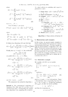
j=1 (1) Input data: x i (0) ∼ (d i (0), f , g ) for
i i
ν i = 1, . . . , ν.
X
f ˜ [t−1] = |w ij |k(f [t−1] , g [t−1] , sgn(w ij )), (2) Input parameters: T, ⃗p, W, ⃗q.
i j j
j=1 (3) Output: x i (T) ∼ (d i (T), f [T] , g [T] ) for
ν i i
[t−1] X [t−1] [t−1] i = 1, . . . , ν.
˜ g i = |w ij |k(g j , f j , sgn(w ij )), (4) For t = 1 to T :
j=1 (5) For i = 1 to ν :
(47)
˜
(a) Calculate z i (t − 1) ∼ (d i (t −
for t = 1, . . . , T − 1. ˜ [t−1] [t−1]
1), f , ˜g ) using Equation (47).
i i
From Corollary 1, we obtain ˜ ˜ [t−1] [t−1]
˜
˜
˜
(b) Calculate (d i (t−1), f i , ˜g i ) us-
˜ ˜ [t−1]
˜
˜ [t−1]
˜
∇ x i (t) = q i (z i (t−1)) ∼ (d i (t−1), f , ˜g ), ing Equation (49).
α i
i i
[t]
[t]
(48) (c) Calculate x i (t) ∼ (d i (t), f , g )
i i
using Equation (51).
T
where (6) Return ⃗x(T) = [x 1 (T), . . . , x ν (T)] .
˜
˜
˜
d i (t − 1) = q i (d i (t − 1)),
˜ [t−1] ˜ ˜ ˜ [t−1] Algorithm 1. Fuzzy solution of System (2)
˜
˜
f (r) = d i (t − 1) − q i (d i (t − 1) − f (r)),
i i
˜
˜
˜
˜ i [t−1] (r) = q i (d i (t − 1) + ˜g i [t−1] (r)) − d i (t − 1). 5. Illustrations and examples
˜ g
(49)
In this section, we present simpler examples to
It follows from Equations (34) and (32) that
ensure understanding of the analysis and notation
!
t−1
⃗ α X Γ(t − s − ⃗α) used throughout this paper. The first example de-
⃗
⃗x(t) = ⃗x(s) ⊕⃗q(⃗z). tails the implementation of Algorithm 1 for a 2D
Γ(1 − ⃗α) Γ(t − s + 1)
s=0 IFDS. The second example demonstrates an ap-
(50)
plication of the proposed incommensurate RNN
Finally, since α i ≥ 0 and t > 1, the coefficients
for local prediction of time series. These exam-
α i Γ(t − s − α i ) ples include the necessary computations to train
Γ(1 − α i ) Γ(t − s + 1) the incommensurate RNN and to obtain the in-
are positive for s = 0, . . . , t − 1. Thus, commensurate order ⃗α.
t−1
α i X Γ(t − s − α i )
d i (t) = d i (s)
Γ(1 − α i ) Γ(t − s + 1) 5.1. Illustrative example
s=0
˜ We consider a 2D NN. Let us consider
˜
+ d i (t − 1),
x 1 (0)(w) =
t−1
[t] α i X Γ(t − s − α i ) [s] 2 2
f (r) = f (r) 1 − (w − d 1 ) /ϵ , w ∈ [−ϵ + d 1 , d 1 + ϵ],
i Γ(1 − α i ) Γ(t − s + 1) i
s=0 0, oth.,
˜ [t−1] (52)
˜
+ f (r),
i
and
t−1
[t] α i X Γ(t − s − α i ) [s] x 2 (0)(w) =
g (r) = g (r)
i i
Γ(1 − α i ) Γ(t − s + 1) 
s=0  1 + (w − d 2 )/ϵ, w ∈ [−ϵ + d 2 , d 2 ], (53)
˜
+ ˜g [t−1] (r), 1 − (w − d 2 )/ϵ, w ∈ [d 2 , d 2 + ϵ],
i
 0, oth.,
(51)
T
and ⃗x(t) = [x 1 (t), . . . , x ν (t)] . where d 1 , d 2 and ϵ > 0 are real numbers. Figure
1 demonstrates these membership functions for
We summarized the method in Algorithm 1. d 1 = 1, d 2 = 2, and ϵ = 1. To find the boundaries
of C x 1 (0) (r), we solve the inverse problem
Remark 4. The computational complexities of 2 2
1 − (w − d 1 ) /ϵ = r
Equations (47), (49), and (51) are O(ν), O(ν),
and thus the boundaries are
and O(νt) for each t. Consequently, the complex- √
ity of Algorithm 1 for computing ⃗x(t) is O(νt(t − w = d 1 ± ϵ 1 − r.
618