Page 78 - IJOCTA-15-4

B. Shiri et.al. / IJOCTA, Vol.15, No.4, pp.610-624 (2025)
we can compute the derivative with respect to α i ,
3.5
yielding
3
∂
2.5 −(1−⃗α)
O x i (t − 1)
∂α k
2
x 1 (t) t−1 t−s−1 t−s−1
1.5 X 1 X Y
= δ ki (j − α i )x i (s).
1 (t − s)!
s=0 r=0 j=0
0.5 j̸=r
(64)
0
0 5 10 15 20 25 30 35
Therefore, the rate of change of x i with respect
t
to α i can be calculated recursively by
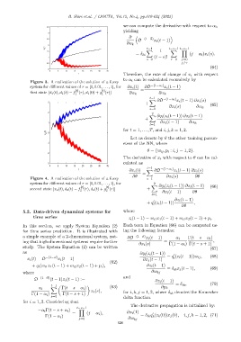
Figure 3. A realization of the solution of a fuzzy
system for different values of r = [0, 0.01, . . . , 1], for ∂x i (t) ∂O −(1−α i ) x i (t − 1)
[t] [t] =
first state [d 1 (t), d 1 (t) − f (r), d 1 (0) + g (r)]
1 1 ∂α k ∂α k
t−1 −(1−α i )
X ∂O x i (t − 1) ∂x i (s)
3 +
∂x i (s) ∂α k (65)
s=1
2 2
X ∂q i (z i (t − 1)) ∂x l (t − 1)
+
1 ∂x l (t − 1) ∂α k
l=1
for t = 1, . . . , T, and i, j, k = 1, 2.
x 2 (t) 0
Let us denote by θ the other training param-
-1 eters of the NN, where
θ = {w ij , p i : i, j = 1, 2}.
-2
The derivative of x i with respect to θ can be cal-
-3 culated as
0 5 10 15 20 25 30 35
t−1
t ∂x i (t) X ∂O −(1−α i ) x i (t − 1) ∂x i (s)
=
∂θ ∂x i (s) ∂θ
Figure 4. A realization of the solution of a fuzzy s=1
system for different values of r = [0, 0.01, . . . , 1], for 2
X ∂q i (z i (t − 1)) ∂x l (t − 1)
[t] [t] (66)
second state [x 2 (t), d 2 (t) − f (r), d 2 (t) + g (r)] +
2 2 ∂x l (t − 1) ∂θ
l=1
∂z i (t − 1)
′
+ q (z i (t − 1)) ,
i
∂θ
5.2. Data-driven dynamical systems for where
time series z i (t − 1) = w i1 x 1 (t − 1) + w i1 x 2 (t − 1) + p i .
In this section, we apply System Equation (2) Each term in Equation (66) can be computed us-
for time series prediction. It is illustrated with ing the following formulas:
a simple example of a 2-dimensional system, not- ∂O −(1−⃗α) x i (t − 1) α i Γ(t − s − α i )
ing that high-dimensional systems require further ∂x i (s) = Γ(1 − α i ) Γ(t − s + 1) ,
study. The System Equation (2) can be written (67)
as ∂q i (z i (t − 1)) ′
i
x i (t) = O −(1−⃗α) x i (t − 1) ∂x j (t − 1) = q (z i (t − 1))w ij , (68)
(62)
+ q i (w i1 x 1 (t − 1) + w i2 x 2 (t − 1) + p i ), ∂z i (t − 1)
= δ ik x j (t − 1), (69)
where ∂w kj
O −(1−⃗α) (t − 1)x i (t − 1) := and
∂z i (t − 1)
= δ ik , (70)
t−1 (63)
α i X Γ(t − s − α i ) ∂p k
x i (s),
Γ(1 − α i ) Γ(t − s + 1) for i, k, j = 1, 2, where δ ik denotes the Kronecker
s=0 delta function.
for i = 1, 2. Considering that
The derivative propagation is initialized by:
t−s−1
−α i Γ(t − s + α i ) Y
= (j − α i ), ∂x i (1) ′
Γ(1 − α i ) = δ ik q (z k (0))x j (0), i, j, k = 1, 2, (71)
k
j=0 ∂w kj
620