Page 79 - IJOCTA-15-4

Analysis and analytical solution of incommensurate fuzzy fractional nabla difference systems...
and
0.8
∂x i (1) ′
= δ ij q (z i (0)), i, j = 1, 2. (72) 0.6
i
∂p j
Here, T represents the memory length of the NN. i 0.4
The incommensurate NN Equation (62) is i 0.2
⃗
trained to obtain ⃗x(T). Inputs are ⃗x {s} (0) = i(s) C x i (2) (r)=[d [2] -f [2] (r),d [2] +g [2] (r)] i i 0
for s = 0, . . . , n, (where n is the number of data
points). In time series analysis, this can be inter- -0.2
preted as predicting the time series at s + T. -0.4
{s} {s}
The goal is x (T) to match real data y ,
i i -0.6
⃗
Corresponds to predicting i(s + c), (with c = 1 or 0 0.2 0.4 r 0.6 0.8 1
c = T). As is conventional, the training energy
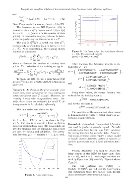
function is minimized: Figure 6. The fuzzy output for fuzzy input data at
m 2 s = 365. The expected value is
Train 1 X X {s} {s} 2 ⃗y(365) = [0.5090, −0.4804] T
E = (x (T) − y ) ,
m i i
s=1 i=1
where m denotes the number of training data After training, the following weights is ob-
points. The derivative of the training energy is: tained for T = 2 :

m
{s}
2
dE Train 2 X X {s} {s} dx (T) 0.9662264009849 −0.0067547002337
= (x (T) − y ) i W = −0.0067547423047 0.9662262855277 ,
dθ m i i dθ
s=1 i=1
0.007754739375402
To train the NN, we use a mini-batch SGD ⃗ p = 0.007754742992966 ,
method 29 combined with the ADAM optimization
and
algorithm. 0.1506754746276
⃗ α = .
Remark 5. As shown in the prior example, even 0.0993245241422
minor input value deviations can cause significant Using these values, the energy function was
output variations when T is large. Moreover, in- reduced for the training data to
creasing T may raise computational costs. No- Train
E = 0.0050824858689,
tably, these issues are mitigated for small T, al-
lowing results to be calculated efficiently. and for the test data to
Test
E = 0.005257048048326.
The time series data described by
The precision of the random test data points

cos(0.02t)
⃗y(t) = 0.01t 0.01t is demonstrated in Table 4, which shows an ac-
(e − 2)/(1 − 2e )
ceptable local prediction.
for t = 1, . . . , 367, is used, as shown in Fig-
ure 5. The aim is to provide a local prediction
Remark 6. A hyperbolic (non-periodic) function
based on previous local data. 240 data points are
was used to predict a periodic signal. Periodic
used for training and the remaining data points
activation functions like sin may better minimize
are used for testing and validation. The activa-
the energy function for periodic data. However,
tion function q i (t) = tanh(t) i = 1, 2, is used.
real-world scenarios often require a single model
1 to handle diverse datasets, making it valuable to
0.8 achieve good results with a fixed activation func-
tion.
0.6
y
0.4 1
y
2
0.2
Finally, Algorithm 1 is used to obtain the
y 0
fuzzy output of this RNN for fuzzy input data
-0.2
at t = 365, with ϵ = 0.1 and shape functions de-
-0.4
fined by Equations (55) and (57). Figure 6 shows
-0.6
C ⃗x(T) (r).
-0.8
The real outputs are ⃗y(365) =
-1
T
0 50 100 150 200 250 300 350 400 [0.5090, −0.4804] . We find that the fuzzy results
t
still distinguish these two values, even though
Figure 5. Time series data input uncertainty introduces ambiguity.
621