Page 26 - MSAM-1-4

Materials Science in Additive Manufacturing Process optimization of SEBM IN718 via ML

and random orientation, as shown in Figure 1C. The where U is acceleration voltage (V), and I represent
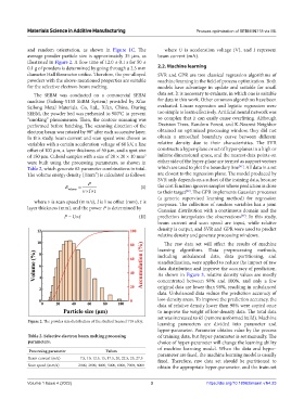
average powder particle size is approximately 35 μm, as beam current (mA).
illustrated in Figure 2. A flow time of 12.0 ± 0.1 s for 50 ±
0.1 g of powders is determined by going through a 2.5 mm 2.2. Machine learning
diameter Hall flowmeter orifice. Therefore, the pre-alloyed SVR and GPR are two classical regression algorithms of
powders with the above-mentioned properties are suitable machine learning in the field of process optimization. Both
for the selective electron-beam melting. models have advantage in update and suitable for small
The SEBM was conducted on a commercial SEBM data set. It is necessary to evaluate, in which one is suitable
machine (Sailong-Y150 SEBM System) provided by Xi’an for data in this work. Other common algorithms have been
Sailong Metal Materials. Co, Ltd., Xi’an, China. During evaluated. Linear regression and logistic regression were
SEBM, the powder bed was preheated to 900°C to prevent too simple to learn effectively. Artificial neural network was
“smoking” phenomenon. Then, the contour scanning was so complex that it can easily cause overfitting. Although
performed before hatching. The scanning direction of the Decision Trees, Random Forest, and K-Nearest Neighbor
electron beam was rotated by 90° after each successive layer. obtained an optimized processing window, they did not
In this study, beam current and scan speed were chosen as obtain a smoothed boundary curve between different
variables with a certain acceleration voltage of 60 kV, a line relative density due to their characteristics. The SVR
offset of 100 μm, a layer thickness of 50 μm, and a spot size constructs a hyper-plane or set of hyper-planes in a high or
of 150 μm. Cuboid samples with a size of 20 × 20 × 10 mm infinite dimensional space, and the nearest data points on
3
were built using the processing parameters, as shown in either side of the hyper-plane are termed as support vectors
[41]
Table 2, which generate 63 parameter combinations in total. which are used to plot the boundary line . All data in a set
The volume energy density (J/mm³) is calculated as follows: are closest to the regression plane. The model produced by
SVR only depends on a subset of the training data, because
P
E volume vl t (I) the cost function ignores samples whose prediction is close
to their target . The GPR implements Gaussian processes
[42]
(a generic supervised learning method) for regression
where v is scan speed (mm/s), l is line offset (mm), t is purposes. The collection of random variables has a joint
layer thickness (mm), and the power P is determined by Gaussian distribution with a continuous domain and the
P = U×I (II) prediction interpolates the observations . In this study,
[37]
beam current and scan speed are input, while relative
density is output, and SVR and GPR were used to predict
relative density and generate processing windows.
The raw data set will affect the results of machine
learning algorithms. Data preprocessing methods,
including unbalanced data, data partitioning, and
standardization, were applied to reduce the impact of raw
data distribution and improve the accuracy of prediction.
As shown in Figure 3, relative density values are mostly
concentrated between 98% and 100%, and only a few
original data are lower than 98%, resulting in unbalanced
data. Unbalanced data reduce the prediction accuracy of
low-density areas. To improve the prediction accuracy, the
data of relative density lower than 98% were copied once
to improve the weight of low-density data. The total data
set was increased to 65 (remove unformed build). Machine
Figure 2. The powder size distribution of the studied Inconel 718 alloy.
learning parameters are divided into parameter and
hyper-parameter. Parameter obtains value by the process
Table 2. Selective electron beam melting processing of training data, but hyper-parameter is set manually. The
parameters. choice of hyper-parameter will change the learning ability
of machine learning model. When the data and hyper-
Processing parameter Values
Beam current (mA) 7.5, 10, 12.5, 15, 17.5, 20, 22.5, 25, 27.5 parameter are fixed, the machine learning model is usually
fixed. Therefore, raw data set should be partitioned to
Scan speed (mm/s) 2000, 3000, 4000, 5000, 6000, 7000, 8000 obtain the appropriate hyper-parameter, and the train-set

Volume 1 Issue 4 (2022) 3 https://doi.org/10.18063/msam.v1i4.23