Page 108 - AJWEP-v22i2

Ghasemi, et al.

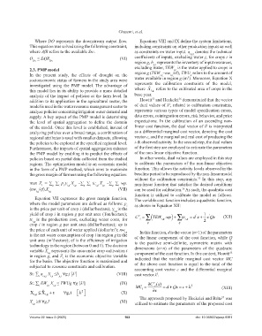
Where DO represents the downstream output flow. Equations VIII and IX define the system limitations,
This equation was solved using the following constraint, including constraints on other production inputs as well
where AfR refers to the available Src. as constraints on water input. a denotes the technical
i,g,j
O ≤ SAfR (VI) coefficients of inputs, excluding water j, for crops i in
Src
Src
region g, b represents the inventory of input resources,
g,j
2.3. PMP model excluding water, TEW is the water applied to crops in
i,g
In the present study, the effects of drought on the region g (TEW =nw /ef), TWU refers to the amount of
i,g
i,g
g
3
socioeconomic status of farmers in the study area were water available in region g (m ). Moreover, Equation X
investigated using the PMP model. The advantage of represents the calibration constraints of the model,

this model lies in its ability to provide a more detailed where X refers to the cultivated area of crops in the
ig,
analysis of the impact of policies at the farm level. In base year.
56
55
addition to its application in the agricultural sector, the Howitt and Heckelei demonstrated that the vector
2
model is used in the water resource management sector to of dual values of λ , related to calibration constraints,
analyze policies concerning irrigation water demand and represents various types of model specification errors,
supply. A key aspect of the PMP model is determining data errors, cointegration errors, risk behavior, and price
the level of spatial aggregation to define the domain expectations. In the calibration of an ascending non-
2
of the model. Once this level is established, instead of linear cost function, the dual vector of λ is interpreted
analyzing policies over a broad range, a combination of as a differential marginal cost vector, denoting the cost
regional attributes is used with smaller datasets, allowing vector c, and the marginal and real cost of producing the
the policies to be explored at the specified regional level. i-th observed activity. In the second step, the dual values
Furthermore, the impacts of spatial aggregation enhance of the first step are employed to estimate the parameters
the PMP model by enabling it to predict the effects of of the non-linear objective function.
policies based on partial data collected from the studied In other words, dual values are employed in this step
regions. The optimization model is an economic model to calibrate the parameters of the non-linear objective
in the form of a PMP method, which aims to maximize function. This allows the activity levels observed in the
the gross margin of farmers using the following equation: baseline period to be reproduced by the non-linear model
without the calibration constraints. In this step, any
55
max Z = ∑ ∑ p .y .X –∑ ∑ tc .X –∑ ∑ wp. non-linear function that satisfies the desired conditions
1
i,g
i
g
i,g
i
g
i,g
g
i
i,g
i
(nw /ef).X i,g (VII) can be used for calibration. As such, the quadratic cost
56
i,g
function is utilized to calibrate the model as follows.
Equation VII expresses the gross margin function, The variable cost function includes a quadratic function,
where the model parameters are defined as follows: p as shown in Equation XII:
i
is the price per unit of crop i (dollar/hectare); y is the
i,g
yield of crop i in region g per unit area (Ton/hectare); C = ( ∑ ´ 1 ´ (XII)
v
tc is the production cost, excluding water costs, for i TEW . wp) + ∑ tc ig , = dx + 2 xQx
ig ,
i,g
crop i in region g per unit area (dollar/hectare); wp is g g
the price of each unit of water applied (dollar/m ); nw i,g
3
is the net water consumption of crop i in region g in the In this function, d is the vector (n×1) of the parameters
unit area (m /hectare); ef is the efficiency of irrigation of the linear component of the cost function, while Q
3
technology in the region (between 0 and 1). The decision is the positive semi-definite, symmetric matrix with
variable X represents the area under crop cultivation i dimensions (n×n) of the parameters of the quadratic
55
i,g
in region g, and Z is the economic objective variable component of the cost function. In this context, Howitt
1
for the basin. The objective function is maximized and indicated that the variable marginal cost vector MC
subjected to resource constraints and calibration. of the above cost function is equal to the total of the
accounting cost vector c and the differential marginal
St: ∑ a X ≤b ∀g,j [λ ] (VIII) cost vector λ .
1
2
i,g
i,g,j
i
g,j
St: ∑ EW X ≤ TWUg ∀g [λ ] (IX) ∂ v x
1
i i,g i,g MC = C () = d + Qxc=+ λ 2 (XIII)
i
i

X ≤ X + ε ∀ gi, λ 2  (X) x ∂
ig, ig,   57
The approach proposed by Heckelei and Britz was
X ≥0 ∀g,I (XI) utilized to estimate the parameters of the proposed cost
i,g
Volume 22 Issue 2 (2025) 102 doi: 10.36922/ajwep.8381