Page 32 - BH-2-2

Brain & Heart Predictive modeling using electroencephalogram

limited or interpretability is important. Choosing the Table 2. K‑size analysis
best model requires careful consideration of the features
of the dataset, the computational limitations, and the Subject Components k=1 k=4 k=7 k=9 k=11
requirements for interpretability so that the model selected Subject 1 Band power 47.8 54.7 58.2 60.2 62.5
closely matches the particular requirements of the EEG Average 34.5 42.8 44.6 50.3 52.4
signal processing task. RMS 65 68.4 72.3 76.2 70
The BCI IV Competition-I dataset may not be entirely Subject 2 Band power 46.2 48.4 49 51.2 54.6
representative of the general population despite offering Average 48.8 46.6 44.1 45.4 50
insightful information on the processing and classification RMS 52 53.3 56.7 54.4 60.2
of EEG signals. Thus, to evaluate the generalizability Subject 3 Band power 64.6 62.9 61 60.1 58.2
and performance of models trained on such benchmark Average 55.2 50 52.2 52.5 59.1
datasets in real-world applications, comprehensive
evaluation and validation, including cross-validation and RMS 62 67.2 70.2 68.3 65
testing on independent datasets, are necessary. Careful Abbreviation: RMS: Root-mean square.
validation is required to determine the best classification
technique with better parameters. The k-fold cross- Table 3. Principal component analysis functions analysis
validation strategy is best because it employs all of the Subject Components Linear Kernel RBF kernel
data trails for both training and testing, which is especially
important given the small sample size. It is possible that Subject 1 Band power 65.2 65.2 63.1
using different techniques will result in an insufficiently Average 42.3 42.3 42.5
precise validation error. When there are many variables in RMS 68.1 72.6 70.4
the ML method, model selection can be critical. The best Subject 2 Band power 52.1 52.1 48
model can be selected by tweaking individual features in Average 42 42 46.7
isolation. However, the accuracy of classification when RMS 64 64 62.2
employing different models may differ from one individual Subject 3 Band power 51 51 48.4
to the next and from one data set to the next. Using
solely MATLAB’s built-in ML and statistics toolboxes, Average 56.3 56.3 47.4
we conducted the following analysis. All feature vectors RMS 72.2 72.2 74.6
were utilized during both the training and testing phases, Abbreviations: RBF: Radial basis function; RMS: Root-mean square.
employing k-fold cross-validation techniques.
4.2.1. K-nearest neighbors
Table 2 demonstrates that a well-trained classifier for the
sorts of signals utilized is often produced using the KNN
method to the dataset and extracting features with different
k-values.
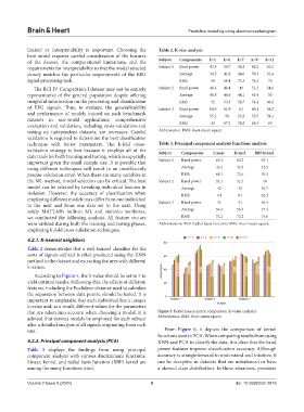
According to Figure 5, the k-value should be set to 7 to
yield optimal results. Following this, the effects of different
features, including the Euclidean distance used to calculate
the separation between data points, should be tested. It is
important to emphasize that each individual has a unique
k-value and, as a result, different values for the parameters
that are taken into account when choosing a model. It is Figure 5. Performance metric comparison (k-value analysis).
advised that various models be employed for each subject Abbreviation: RMS: Root-mean square.
after a detailed analysis of all signals originating from each
one. From Figure 6, it depicts the comparison of kernel
functions used in PCA. When comparing results from using
4.2.2. Principal component analysis (PCA) KNN and PCA to classify the data, it is clear that the band
Table 3 displays the findings from using principal power features improve classification accuracy. Although
component analysis with various discriminant functions. accuracy is straightforward to understand and intuitive, it
Linear, kernel, and radial basis function (RBF) kernel are can be deceptive in datasets that are unbalanced or have
among the many functions tried. a skewed class distribution. In these situations, precision

Volume 2 Issue 2 (2024) 8 doi: 10.36922/bh.2819