Page 33 - BH-2-2

Brain & Heart Predictive modeling using electroencephalogram

and recall offer more information about the performance
of the classifier but might not be as effective at capturing
the overall classification performance as accuracy. The
aforementioned tabulated results demonstrate that it
would be unrealistic to assume that a single classification
model would be effective across multiple datasets obtained
from multiple test subjects under multiple experimental
conditions and over time. The algorithm may not be able
to accurately fit the available data into the model, or a lack
of training data may be to blame for some models’ low
performance for some subjects.

4.2.3. Neural networks
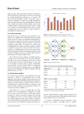
Figure 6. Performance metric comparison: Function analysis.
Through the process of learning a representation of the Abbreviations: RBF: Radial basis function; RMS: Root-mean square.
input at the hidden layers, multilayer neural networks
can be utilized for feature learning before being applied to
classification or regression. The majority of neural networks
will adjust the model’s parameters iteratively in response to
a training sample. With each iteration, the cost function,
or classification error, should get smaller. Figure 7 displays
a simplified version of the neural network with just one
input layer, two hidden layers, and one output layer. Results,
however, have been confirmed through testing with varying
densities of hidden layer neurons. Normal data present the
network with a 400-element input vector.
The network may not be able to accurately describe a
test input vector, even though it has learned a model that
correctly characterizes the majority of the data in all of
the input vectors. Based on these findings, it is clear that Figure 7. Neural network structure.
as the number of hidden neurons grows, classification
accuracy suffers. Due to the finite number of training input Table 4. Neural network with different hidden neurons
vectors, models with more hidden units are more likely to
experience over-fitting issues. Table 4 illustrates NN with Hidden units=2 400 600 800
different hidden neurons. Subject 1 78.3 76.2 74.5
4.3. Performance analysis Subject 2 70.1 68.6 62.8
Subject 3 74.4 72.9 71.2
The classification results for the experimental data are
presented in Table 5, demonstrating that the KNN
algorithm can accurately classify emotional states based on Table 5. Accuracy analysis
the EEG data. Both PCA and NN also endeavor to categorize Subject KNN PCA NN
samples into subsets based on specific criteria. However, it
is possible that the EEG data related to emotional states Subject 1 85.6 36.3 28.1
may be clustered without a clear delineator between the Subject 2 86.8 34.2 30.3
various types of data available to us. Subject 3 82.3 28.8 31
From Figure 8, it can be concluded that the KNN Abbreviations: KNN: K-nearest neighbor; NN: Dual-layer neural
network; PCA: Principal component analysis.
method is the most appropriate for categorizing the data.
A test is done to confirm the claim. The first step involved
grouping the vehicle parameters gleaned from driving then use a KNN classifier to assign each recording to one
the simulated car into one of four categories representing of four possible mental states. High arousal and a favorable
four distinct human driving styles: cautious, aggressive, valence describe the alert mental state.
inexpert, and relaxed. The second step is to record subjects’ An eager or enthusiastic person is viewed as a keen
electrical brain activity while they operate the vehicle, and operator. The operator is familiar with the vehicle’s

Volume 2 Issue 2 (2024) 9 doi: 10.36922/bh.2819