Page 67 - GHES-1-2

Global Health Econ Sustain Stochastic modeling of age at menopausal

α − 1  α  θ
α  x   x    α  λ 
x 
fx () = ββ exp −    , for x > 0 (6)       

 
3
  
β

 


β

 
Fx () =−   1−      (11)
1
6
α
   x   
  x  α    1+    
β
 
Fx () =− exp −    , for x > 0 (7)      
1

3

β
  


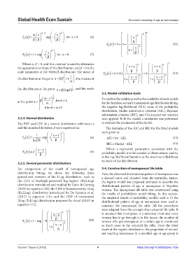
Where α, β > 0, and this constant is used to determine  α   α  2
γ
the appearance or shape of the distribution, and β > 0 is the    x −       x − γ   
scale parameter of the Weibull distribution. The mean of Fx () = ( 1+ )λ   β     β  
 (12)

 − λ 
α
α
 1  6   x −     x −  
γ
γ
the distribution at the point x = βΓ   1+ α   , the median of  1+   β    1 +   β  






1
the distribution at the point x = ( β log ) α , and the mode
2
3.3. Model validation tools
 1
 β  α− 1 α  , for α> 1 To confirm the validity as well as the suitability of used models

at the point x =      α . for the Nepalese women’s menopausal age distribution fitting,

  0 for 0 < α ≤ 1 the negative log-likelihood (NLL) value of the probability
distribution, Akaike information criterion (AIC), Bayesian
information criterion (BIC), and Chi-squared test statistics
3.2.4. Normal distribution were applied. To fit the model, a simulation was performed
The PDF and CDF of a normal distribution with mean γ to estimate the parameters of the model.
and the standard deviation β were expressed as: The formulae of the AIC and BIC for the fitted models
1   x −γ  2  were given as:
f ( ) x = exp −    (8) AIC 2 – 2 LL= ν (13)

4
2π  β  β    
BIC Ln(n) – 2 LL= ν (14)
 x −  Where ν represents parameters associated with the
γ
Fx () = ƒ   β   (9) probability model, n is the number of observations, and LL
4
is the log-likelihood function at the maximum likelihood
estimate of the distribution.
3.2.5. Several parameter distributions
For comparison of the result of menopausal age 3.4. Construction of menopausal life table
distribution fitting, we chose the following three Here, the observed distributional pattern of menopause was
generalized versions of the LLog distribution, such as a skewed curve and deviated from the normality. Hence,
the CDF of Rayleigh-generated log-logistic (RGLLog) the logistic model was proposed and used to describe the
distribution introduced and studied by Gaire & Gurung distributional pattern of age at menopause of Nepalese
(2023) in equation (10); the CDF of Kumaraswamy LLog women. The menopausal life table was constructed using
(KuLLog) distribution introduced by De Santana et al. the results of probabilistic model fitting. In this section,
(2012) in equation (11); and the CDF of transmuted the empirical results of probability models used to fit the
LLog (TrLLog) distribution proposed by Aryal (2013) in distributional pattern of age at menopause were used to
equation (12). construct the menopausal life table. All the procedures
  α  2  were adopted from the concept of an actuarial life table. It
   x −γ    is assumed that menopause is a universal event and every
    β     woman has to go through it in life; hence, the number of
F 5 ( ) x = −    α    (10) women who got menopause at a certain age is considered
1 exp −θ
   x −γ    as death cases in the actuarial life table. From the fitted
 1+     β    
     result of the logistic distribution, the proportion of women
not reaching menopause in a specified age or age group is
Volume 1 Issue 2 (2023) 4 https://doi.org/10.36922/ghes.1239