Page 174 - IJOCTA-15-1

Y. Olmez et al. / IJOCTA, Vol.15, No.1, pp.166-182 (2025)
2. Metaheuristic methods 2.1. Political optimizer

This study presents an investigation of control pa- The Political Optimization (PO) algorithm, in-
rameter determination for the recent metaheuris- spired by political processes, was proposed by As-
tic methods which are PO, EO, AO, FDA, CO, gari et al in 2020. 24 All stages of political par-
ARO, GJO, GOA, and POA. These methods ties were modeled and their mathematical mod-
are compared with older metaheuristics, namely els were derived. The initial population is cre-
Whale, Grey Wolf, Crow Search, Covariance Ma- ated by dividing it into parties and electoral dis-
trix Adaptation Evolution Strategy, and Flower tricts. The algorithm is divided into five phases:
Pollination optimization algorithms. Table 1 party formation, voter allocation, election cam-
presents the details of the considered methods. paign, party change, and election affairs. Each
The details of the methods, including the al- population identifies one member and its votes
gorithm’s inspiration, published years and jour- are represented by the fitness values. Each party
nals, and author names are provided in Table 1. embodies a potential solution to the issue.
The determined methods for analyzing control pa- The main equation for the position update is
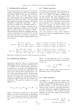
rameter determination are selected from the last found in the election campaign section, as given
four years and they are inspired by various ar- below Eqs. (1-2):
eas such as nature-inspired, physic-inspired, and
socio-inspired.

 ∗ ∗ j j j ∗ j j ∗
m + r(m − p (t)), if p (t − 1) ≤ p (t) ≤ m or p (t − 1) ≥ p (t) ≥ m
 i,k i,k i,k i,k i,k
∗
∗
∗
P j (t + 1) = m + (2r − 1)|m − p j (t)|, if p j (t − 1) ≤ p j (t) ≤ m or p j (t − 1) ≥ p j (t) ≥ m ∗ (1)
i,k i,k i,k i,k i,k i,k
 ∗ ∗ j j j ∗ j j ∗
m + (2r − 1)|m − p i,k (t − 1)|, if p i,k (t − 1) ≤ p i,k (t) ≤ m or p i,k (t − 1) ≥ p i,k (t) ≥ m

 ∗ ∗ j j j ∗ j j ∗
m + (2r − 1)|m − p (t)|, if p (t − 1) ≤ p (t) ≤ m or p (t − 1) ≥ p (t) ≥ m
 i,k i,k i,k i,k i,k
∗
∗
P j (t + 1) = p j (t − 1) + r(p j (t) − p j (t − 1)), if p j (t − 1) ≤ m ≤ p j (t) or p j (t − 1) ≥ m ≥ p j (t) (2)
i,k i,k i,k i,k i,k i,k i,k i,k
 j j j j j
m + (2r − 1)|m − p i,k (t − 1)|, if m ≤ p i,k (t − 1) ≤ p i,k (t) or m ≥ p i,k (t − 1) ≥ p i,k (t)
 ∗ ∗ ∗ ∗
j
Where p i,k (t) indicates the jth member of the ith party with d-dimension.
2.2. Equilibrium optimizer Where t 0 is the initial time and t is a function
linearly decreasing and calculated as the follow-
ing Eq. (5):
Equilibrium Optimizer (EO) is a physics-based
it
optimization method developed by Faramarzi et it a 2 max it (5)

al. in 2020. 25 In the updating stages, individuals t = 1 −
max it
are guided by a set of rules to an equilibrium po-
sition where the solutions are equally good. The Where a 2 is the constant value related to the ex-
method was designed with inspiration from con- ploitation ability of the algorithm.
trol volume mass balance models. In these mod-
els, starting from the rule that the total mass of a
substance is constant, the population is directed
toward the position where the total fitness is in 2.3. Aquila optimizer
equilibrium. The particles’ positions are revised
Abualigah et al. developed the Aquila Opti-
using Eq. (3): mizer (AO), a population-based metaheuristic al-
gorithm, in 2021. 26 It was inspired by the Aquila’s
hunting behavior. It has four stages in the up-
r
⃗
⃗
⃗x = ⃗x eq + (⃗x − ⃗x eq ) · F + · (1 − F) (3) dating process, which are expanded exploration,
⃗ narrowed exploration, expanded exploitation, and
λV
narrowed exploitation. The proposed updating
Where x denotes the concentration of the control equations at these four stages are given respec-
volume, ⃗x eq is the concentration at an equilibrium tively as follows:
state. λ is a random vector in [0-1]. F denotes the
exponential term and can be calculated with Eq. it
(4): (x 1 (t + 1) = x best (t) . 1 −
max it (6)
(F = e −λ(t−t 0 ) ) (4) + (x m (t) − x best (t) .r)
168