Page 175 - IJOCTA-15-1

Recent metaheuristics on control parameter determination
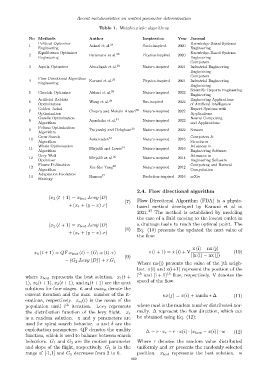
Table 1. Metaheuristic algorithms

No Methods Author Inspiration Year Journal
Political Optimizer Knowledge-Based Systems
1 Askari et al. 24 Socio-inspired 2020
Engineering Engineering
Equilibrium Optimizer Knowledge-Based Systems
2 Faramarzi et al. 25 Physics-inspired 2020
Engineering Engineering
Computers
3 Aquila Optimizer Abualigah et al. 26 Nature-inspired 2021 Industrial Engineering
Engineering
Computers
Flow Directional Algorithm
4 Karami et al. 27 Physics-inspired 2021 Industrial Engineering
Engineering
Engineering
Scientific Reports Engineering
5 Cheetah Optimizer Akbari et al. 28 Nature-inspired 2022
Engineering
Artificial Rabbits Engineering Applications
6 Wang et al. 29 Bio-inspired 2022
Optimization of Artificial Intelligence
Golden Jackal 30 Expert Systems with
7 Chopra and Mohsin Ansari Nature-inspired 2022
Optimization Applications
Gazelle Optimization Neural Computing
8 Agushaka et al. 31 Nature-inspired 2022
Algorithm and Applications
Pelican Optimization
9 Trojovsk´y and Dehghani 32 Nature-inspired 2022 Sensors
Algorithm
Crow Search 33 Computers &
10 Askarzadeh Nature-inspired 2016
Algorithm Structures
Whale Optimization Advances in
11 Mirjalili and Lewis 34 Nature-inspired 2016
Algorithm Engineering Software
Grey Wolf Advances in
12 Mirjalili et al. 35 Nature-inspired 2014
Optimizer Engineering Software
Flower Pollination 36 Computing and Natural
13 Xin-She Yang Nature-inspired 2012
Algorithm Computation
Adaptation Evolution
14 Hansen 37 Evolution-inspired 2016 arXiv
Strategy
2.4. Flow directional algorithm
(x 2 (t + 1) = x best .Levy (D)
(7) Flow Directional Algorithm (FDA) is a physic-
+ (x r + (y − x) .r) based method developed by Karami et al in
2021. 27 The method is established by modeling
the case of a fluid moving to the lowest outlet in
(x 2 (t + 1) = x best .Levy (D) a drainage basin to reach the optimal point. The
(8) Eq. (10) presents the updated the next value of
+ (x r + (y − x) .r)
the flow:

x (i) − nx (j)
x 4 (t + 1) = QF.x best (t) − (G 1 .x (t) .r) x (i + 1) = x (i) + V (10)
(9) ||x (i) − nx (j)
− (G 2 .Levy (D)) + r.G 1
Where nx(j) presents the value of the jth neigh-
bor. x(i) and x(i+1) represent the position of the
i th and (i + 1) th flow, respectively. V denotes the
where x best represents the best solution. x 1 (t +
speed of the flow.
1), x 2 (t + 1), x 3 (t + 1), and x 4 (t + 1) are the next
solutions for four stages. it and max it denote the
current iteration and the max. number of the it- nx(j) = x(i) + randn ∗ ∆ (11)
erations, respectively. x m (t) is the mean of the
population until t th iteration. Levy represents where rand is the random number distributed nor-
mally. ∆ represent the flow direction, which can
the distribution function of the levy flight. x r
is a random solution. x and y parameters are be obtained using Eq. (12):
used for spiral search behavior. a and δ are the
exploitation parameters. QF denotes the quality
∆ = r · x r − r · x(i) · |x best − x(i)| · w (12)
function, which is used to balance between search
behaviors. G 1 and G 2 are the motion parameter Where r denotes the random value distributed
and slope of the flight, respectively. G 1 is in the uniformly and xr presents the randomly selected
range of [-1,1] and G 2 decreases from 2 to 0. position. x best represents the best solution. w
169