Page 143 - IJOCTA-15-2

E. Karabulut T¨urkseven, E. Gen¸c, and I. Safak / Vol.15, No.2, pp.330-342 (2025)
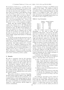
the successors of task 2 is x s = 5 (the only suc- As mentioned in Section 3, the EOD process
cessor task 4 is at position 5). We choose a ran- consists of five stages. The number of tasks in
dom position among the possible options {2, 3, 4}, each stage and the average duration of the stages
′
let’s say we choose the new position x = 2. We are shown in Table 2, demonstrating the size and
place task 2 in position 2, and shift the Activity impact of the problem at hand. Since stages 3
List accordingly to get [0, 2, 1, 3, 4]. Since task and 5 are small both in terms of the number of
2 only has a single mode, we have to choose 1 tasks and duration; meaningful improvement can
again for its mode, and therefore Mode List re- be observed only in stages 1, 2, and 4.
mains as [1, 2, 1, 1, 1]. Given the solution Activity
List = [0, 1, 3, 2, 4] and Mode List = [1, 2, 1, 1, 1]; Table 2. Stage Information
the new solution Activity List = [0, 2, 1, 3, 4] and
Number Average Duration
Mode List = [1, 2, 1, 1, 1] is considered a neighbor.
of Tasks (minutes)
Notice that this random neighbor selection Stage 1 70 26.225
scheme may result in one of the following four Stage 2 80 109.95
outcomes: (1) Activity List is changed, Mode List Stage 3 10 7.575
remains the same, (2) Mode List is changed, Ac- Stage 4 60 103.1
tivity List remains the same, (3) both Activity Stage 5 10 0.425
List and Mode List are changed, and (4) both The first analysis concerns the impact of
scheduling, i.e., the order of tasks, on the
Activity List and Mode List remain the same. In
makespan of the project. The goal of this analy-
the case of outcome (4), the random neighbor se-
sis is not to determine how many threads to al-
lection scheme repeats itself instead of returning
locate to each task; rather use the same thread
identical lists.
allocations that have been used, keep the thread
For details on selecting the parameters for the
usage and duration constant for each task, and
SA algorithm described in Figure 5, the reader is
referred to. 27 In our application, we used C = 2 only solve for the order of execution of tasks. We
adapt our model to solve this problem simply by
chains, where T and n 0 are initialized as 10 and 80
setting the number of modes of each task to one.
respectively. Each chain consists of S = 5 steps,
Due to the variability of task durations each
at each step n s neighbor comparisons are made
(which may or may not result in updating the cur- day, the scheduling decision, which must be made
rent solution), and at the end of each stage s, T is before execution, cannot rely on actual daily du-
updated as T/4, and n s is updated as n s · (1 + s). rations. Instead, for the scheduling problem we
These values are chosen as a result of prelimi- use estimate values for the task durations. Due
nary experiments, to minimize the duration of the to the daily deviation in task durations, the es-
timated makespan and the realized makespan of
search while maintaining solution quality.
each stage may differ significantly.
To provide a fair comparison, we randomly se-
5. Results lected seven days from the range of the daily job
logs (i.e., historical data). For each day, we
We wish to emphasize that the SA algorithm
• solve the optimization problem for each
serves as a solution to our problem that does
stage, where all tasks are restricted to a
not require a commercial solver while achieving
the optimal solution for this specific data set. single mode (which is the existing setting),
Our experiments confirmed that for these spe- and the durations are the estimated task
cific instances, the solutions obtained by SA in- durations based on the median of obser-
deed match the optimal solution found by Gurobi. vations in the daily logs,
Therefore, no further research has been conducted • obtain an order of execution from the op-
for a better heuristic alternative, as SA is both timization problem,
fast enough for this implementation, and reaches • use the realized task durations of that day
the optimal solution. to calculate the makespan of the stage if
it had been executed according to the new
This section provides an analysis of the exist-
ing EOD system and the impact of the MRCSP schedule.
on the proposed EOD process optimization. Our The makespan calculated in this manner is
analysis focuses on three primary aspects: the im- referred to as New Schedule. This value is com-
pact of optimizing only the scheduling decisions, pared with the actual stage durations observed
the impact of scheduling and reassigning resource in the daily logs, referred to as Actual Schedule.
usages (i.e., mode selection), and the impact of Tables 3 - 5 report these values for all 7 days for
resource availabilities. Stages 1, 2, and 4; and the values provided are
338