Page 144 - IJOCTA-15-2

End of day process optimization
in minutes. Since in daily job logs, the start and Next, we analyze the impact of multiple
end times of tasks are given as time stamps in modes in each stage. As studied in critical path
minutes, the values in these tables are prone to analysis, shortening an arbitrary task does not
±1 minute error. necessarily shorten the whole process. Only those
on the critical path have a direct impact on the
Table 3. Impact of Scheduling in Stage 1 project duration. Similarly, providing shorter or
longer modes for arbitrary tasks does not have a
Actual New directly foreseeable outcome. Furthermore, with
Schedule Schedule
different precedence structures in different stages,
Day 1 24 24
Day 2 22 22 the impact of multiple modes is expected to differ
Day 3 21 21 between stages.
Day 4 27 26 For the analysis whose results are displayed
Day 5 20 20 in Table 6, we solve the single mode resource-
Day 6 9 9 constrained scheduling problem to get an esti-
Day 7 8 9
mated duration of each stage without multiple
Table 4. Impact of Scheduling in Stage 2 modes; and the multi-mode resource constrained
scheduling problem to get an estimated dura-
Actual New tion and report the percentage improvement in
Schedule Schedule
Day 1 103 107 makespans. In other words, the values in Ta-
Day 2 109 106 ble 6 are calculated as (multi-mode duration -
Day 3 93 101 single mode duration) / (single mode duration) ·
Day 4 104 98 100. The most significant enhancement occurred
Day 5 90 94 in Stage 1, with an 18% reduction, while the least
Day 6 85 88
Day 7 86 86 effect was noted in Stage 2, with an 8% reduction
in makespan.
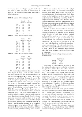
Table 5. Impact of Scheduling in Stage 4
Table 6. Improvement in Stage Makespans with
Multiple Modes
Actual New
Schedule Schedule
Improvement
Day 1 86 86
Stage 1 -18.1%
Day 2 92 86
Stage 2 -7.9%
Day 3 94 86
Stage 4 -15.2%
Day 4 92 84
Note that for this analysis, we have to use
Day 5 72 71
Day 6 78 62 the estimated makespans given by the optimiza-
Day 7 91 72 tion problem, rather than the actual observa-
We observe three different behaviours for the tions, such as the ones that were used in Tables
three stages. In stage 1, seen in Table 3, the ac- 3 - 5. The reason behind this is that although
tual order of execution and the optimized order of we have actual observations for the single-mode
execution are the same; hence stage 1 requires no makespans, we do not have actual observations
assistance for scheduling. In stage 4, seen in Ta- for the multi-modes (i.e. historical data only has
ble 5, the system significantly benefits from opti- the default thread usages, we don’t have any ob-
mized scheduling most of the time (such as days 2, servations of the task under the proposed thread
3, 4, 6, and 7), and in the remaining days the two count selection). Therefore, for fairness, we base
schedules yield almost identical results. The im- the comparison on the optimization problem re-
pact of the scheduling problem in stage 2, seen in sults using the estimations.
Table 4, is uncertain. Due to the discrepancy be- The values in Tables 2 - 6 are generated under
tween the actual task durations and the estimated the existing system parameters with 200 threads
durations used in the optimization problem, the and 15 parallel tasks available. To make the EOD
resulting schedule yields a shorter makespan on process more efficient, one might also consider in-
some days (such as days 2 and 4) and a longer vesting in the infrastructure to increase resource
makespan on others (such as days 1, 3, 5, and availability. However, before this investment, we
6). Paired t-tests conducted to these three groups would like to observe the potential benefit of in-
of schedules, indicate that the mean duration of creasing the resources and understand how effi-
Stages 1 and 2 can be assumed to be identical, ciently we are using the existing resources.
with corresponding p-values of 1 and 0.457, re- Tables 7 - 9 report the estimated makespan
spectively. However the mean durations of Stage of stages 1, 2, and 4 respectively, when MRCSP
4 are statistically different with a p-value of 0.021. is solved with varying resource availabilities. The
339