Page 162 - IJOCTA-15-2

A modified graphical based tuning and performance analysis of second order LADRC . . .

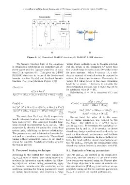
Figure 1. (a) Generalized SLADRC structure, (b) SLADRC 2-DOF structure

The transfer function form of the equations within which controllers can be feasibly selected.
4
is obtained by substituting the controller and ob- For the design of the parameter k, noted that
server gains and the Laplace transform of equa- the typical range between 3 and 10 works better
tion (3) in equation (6). This gives the 2-DOF for most systems. When k exceeds 10, a sub-
SLADRC structure in terms of the feedforward stantial amount of control action is required to
transfer function G FF (s) and feedback transfer achieve the desired performance. Conversely, for
function G FB (s) as (shown in Figure 1(b)) values of k values below 3, the state estimation
tends to be slower. Therefore, to expedite the
G FF (s) = state-estimation process, the k value was set to
its maximum value (k = 10).
2
ω (s + kω c ) 3 Substituting k = 10 in equations (11) and
c
2
2
2 2
2
b 0 s (s + (3kω c + 2ω c ) s + (3k ω + 6kω + ω )) (12),
c
c
c
(11)
2
ω (s + 10ω c ) 3
c
G FB (s) = G FF (s) = (13)
2
2
b 0 s (s + 32ω c s + 361ω )
c

2

2 2

2
kω 3 s 2 k + 6k + 3 + s 2k ω c + 3kω c + k ω
c c
2
2
2
2
2 2
b 0 s (s + (3kω c + 2ω c ) s + (3k ω + 6kω + ω )) G FB (s) = 10ω 3 c 163s + 230ω c s + 100ω c 2 (14)
c
c
c
2
(12) b 0 s (s + 32ω c s + 361ω )
2
c
The controllers G F F and G F B, respectively
Having fixed the value of k, the num-
handle set-point tracking and disturbance rejec-
ber of tuning parameters was reduced to two
tion, respectively. The controller transfer func- (b 0 , & ω c ). The values of b 0 ̸= 0, ∀ b 0 (−∞, ∞)
tions depend on parameters b 0 , k, and ω c . The and (0<ω c <∞). To formulate the analytical ex-
parameter b 0 directly influences the closed-loop pression for b 0 and ω c , it is essential to choose
system gain, exhibiting an inverse relationship. closed-loop design specifications that directly im-
The parameters ω c and k determine the controller pact the time-domain performance and facilitate
pole and zero locations, respectively. The optimal system stability assessment. In line with these cri-
tuning of these parameters relative to the plant is teria, the most suitable design specifications are
crucial for stability. Analytical formulae simplify the PM and ω gc . Notably, the settling time of the
the tuning process. closed-loop system is directly associated with PM.
3. Proposed tuning technique 3.1. Synthesis of tuning parameters
According to the control law, three parameters The PM and ω gc are selected as the design spec-
(b 0 , k, ω c ) must be tuned. The tuning method in- ifications, and the stability of the inner closed-
troduced in this section aims to achieve the follow- loop system was analyzed using the Nyquist plot.
ing objectives: reduce tuning parameters, apply The design objective is to arrive at suitable de-
an inversion formula over the controller, derive sign specifications (PM, ω gc ) and develop an ap-
analytical formulas for tuning parameters based propriate tuning law for the controller parameters
on design specifications, and establish a range (b 0 , ω c ) to achieve the desired performance.
357