Page 167 - IJOCTA-15-2

J. Gunasekaran et.al / IJOCTA, Vol.15, No.2, pp.354-367 (2025)
Table 3. Pros and cons of the proposed tuning approach relative to the existing techniques

System / Existing Techniques from Literature Proposed Technique
Reference
GP 3 [38] Pros
Pros
• Model-based controller design using the IMC technique.
• Partial model information is
• Applicable for second-order and third-order LADRC tuning. sufficient (magnitude and
• Designed for oscillatory systems with time delay. system phase at desired
Cons frequency).
• Closed loop performance sensitive to model mismatch. • Generalized Tuning formulae
• It is difficult to form a generalized solution.
based on PM and ω pc .
• Time-consuming process for selecting an appropriate model.
• Admissible region provides
bound limits for optimization.
[39] Pros • Applicable for most of the SISO
• Designed for generalized integrating systems. systems (Stable, Oscillatory,
• Provides tuning range for LADRC parameters. Unstable, non-minimum phase,
Cons Integrating and others).
• Time taking process due to trial and error approach. • Deals only with Second order
• Difficult to apply this for NMP and underdamped systems. LADRC.

Cons
[20] Pros
• Tuning based on system model approximation as FOPDT. • Difficult to apply on complex
• Provided unique analytical tuning formulae for b 0 , ω c and ω 0 . systems (combination of unstable,
time delay, and
Cons
non-minimum phase systems)
• Model reduction techniques required.
• Time consuming applying for Non-minimum phase and Unstable system. • Iterative method is time
• Two step processes of tuning. consuming.

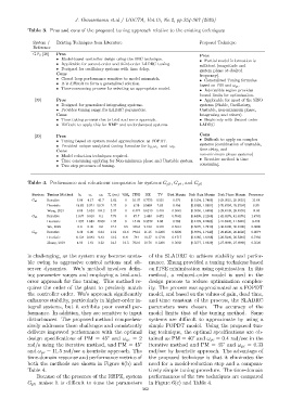
Table 4. Performance and robustness comparison for systems G p3 , G p4 , and G p5
System Tuning Method b 0 ω c ω 0 T s (sec) %M p ITSE ISE TV Disk Margin Disk Gain Margin Disk Phase Margin Frequency
G p3 Iterative 3.86 4.17 41.7 2.82 0 10.37 0.7735 0.315 0.579 [0.5134, 1.7403] [-29.9515, 29.9515] 11.68
Heuristic 18.83 5.921 59.21 2.27 0 8.29 0.5894 2.65 0.456 [0.6289, 1.5901] [-25.6704, 25.6704] 6.99
Wang, 2021 6.05 3.624 104.2 2.97 0 8.474 0.6219 3.418 0.5081 [0.5950, 1.6806] [-28.4939, 28.4939] 14.84
G p4 Iterative 1.937 0.810 8.1 7.79 0 47.7 2.443 0.472 0.7682 [0.4498, 2.2269] [-41.6276, 41.6276] 1.4782
Heuristic 1.937 4.662 46.62 1.35 0 15.29 0.3572 2.98 0.766 [0.4492, 2.2263] [-41.6240, 41.6240] 8.499
Wu, 2022 0.8 0.35 0.6 17.4 0.5 448.8 9.102 0.318 0.5513 [0.5679, 1.7610] [-30.8196, 30.8196] 0.6885
Iterative 6.39 0.90 9.02 11.9 10.6 774.3 11.15 0.1205 0.5899 [0.7072, 1.7140] [-29.4620, 29.4620] 0.8577
G p5
Heuristic 8.134 0.942 9.42 12.2 8.41 744 10.57 0.1718 0.4717 [0.6185, 1.6168] [-26.5246, 26.5246] 0.7493
Zhang, 2019 4.93 1.61 3.22 14.5 16.5 762.6 10.76 0.1266 0.5663 [0.5577, 1.6929] [-27.6989, 27.6989] 0.5526

is challenging, as the system may become unsta- of the SLADRC to achieve stability and perfor-
ble owing to aggressive control actions and ob- mance. Zhang provided a tuning technique based
server dynamics. Wu’s method involves defin- on ITSE minimization using optimization. In this
ing parameter ranges and employing a trial-and- method, a reduced-order model is used in the
error approach for fine tuning. This method re- design process to reduce optimization complex-
quires the order of the plant to precisely match ity. The process was approximated as a FOPDT
the controller order. Wu’s approach significantly model, and based on the values of gain, dead time,
enhances stability, particularly in higher-order in- and time constant of the process, the SLADRC
tegral systems, but it exhibits poor overall per- parameters were chosen. The accuracy of the
formance. In addition, they are sensitive to input model limits that of the tuning method. Some
disturbances. The proposed method comprehen- systems are difficult to approximate by using a
sively addresses these challenges and consistently simple FOPDT model. Using the proposed tun-
delivers improved performance with the optimal ing technique, the optimal specifications are ob-
design specifications of PM = 45° and ω gc = 2 tained as PM = 40° and ω gc = 0.4 rad/sec in the
rad/s using the iterative method, and PM = 45° iterative method and PM = 45° and ω gc = 0.33
and ω gc = 11.5 rad/sec a heuristic approach. The rad/sec by heuristic approach. The advantage of
time-domain response and performance metrics of the proposed technique is that it eliminates the
both the methods are shown in Figure 6(b) and need for a model-reduction step and a compara-
Table 4. tively simple tuning procedure. The time-domain
Because of the presence of the RHPZ, system performances of the two techniques are compared
G p5 makes it is difficult to tune the parameters in Figure 6(c) and Table 4.
362