Page 164 - IJOCTA-15-2

A modified graphical based tuning and performance analysis of second order LADRC . . .

x 2 = (1.1057ω tan (φ c )
!
r

2
+0.5ω (−2.2114 tan (φ c )) + 6.2524
Solving equations (24) and (25) for ω c af-
ter applying the condition given in equation (23)
yields,

(1.1057 tan (φ c )

r 2

2
− 0.5 −2.2114tan (φ c ) + 6.2524 > 0.268
(26)
The admissible range for the phase of the con-
troller (φ c ) with respect to ω c using Equation (26)
(Wolfram Mathematica) becomes:

π π
φ c ϵ (−π, −0.7306π] ∪ − ∪ , π
2, 0.2694π 2
(27)
Similarly, with respect to b 0 using equation
(21) we get,
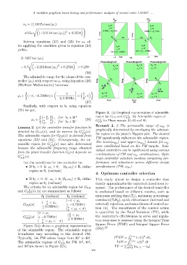
Figure 2. (a) Graphical representation of admissible
π π + −1
− , , for b 0 ∈ R region for G F B and G F B . (b) Admissible region of
φ c ∈ π 2 π 2 − (28) G −1 for Phase margin 30, 60 and 90
2 , − 2 , for b 0 ∈ R F B
Remark 2. 2 The permissible range of ω gc is
Lemma 2. Let the controller transfer function be
denoted by G FB (s), and its inverse by G −1 (s). graphically determined by overlaying the admissi-
FB ble region on the plant’s Nyquist plot. The desired
The admissible region for G FB (s) is derived from
PM significantly influences the admissible region.
equations (23) and (24). Consequently, the ad-
missible region for G −1 (s) was also determined The lower(ω gc l ) and upper (ω gc u ) bounds for ω gc
FB were established based on the PM targets. Indi-
because the admissible frequency range obtained
vidual controllers can be synthesized using various
from the plant transfer function G p (s) depends on combinations of PM and ω gc combinations. Opti-
G −1 (s).
FB mum controller selection involves comparing per-
Let the conditions for the controller be: formance and robustness across different design
• If b 0 > 0 & ω c > 0; (b 0 , ω c ) ∈ R, define specifications (PM, ω gc ).
region as θ 1 (radians)
4. Optimum controller selection
• If b 0 < 0 & ω c > 0; (b 0 , ω c ) ∈ R, define This study aimed to design a controller that
region as θ 2 (radians) closely approximates the expected closed-loop re-
The criteria for an admissible region for G FB sponse. The performance of the desired controller
and G −1 (s) (s) are summarized as follows: is evaluated based on different metrics, such as
FB
θ 1 (radians) θ 2 (radians) minimum settling time(T s ), minimum percentage
overshoot(%M p ), quick disturbance (internal and
π (−π < φ c
(− < φ c
G FB (s) 2 ≤ −0.7306π) external) rejection, and smoothness of control ac-
≤ 0.2694π) π
( < φ c < π) tion (u). The smoothness of the control action
2
is quantified by the Total Variation (TV), while
(π > φ c π
G −1 (s) ≥ −0.7306π) ( < φ c the controller’s effectiveness in servo and regula-
2
FB ≤ 0.2694π)
π
(− > φ c > −π) tory responses is assessed using the Integral Time
2
Figure 2(a) shows a graphical representation Square Error (ITSE) and Integral Square Error
(ISE). 22
of the admissible region. The admissible region
boundaries vary according to the desired PM.
R t sim 2
Typically, the PM values range from 30° to 60°. ITSE = 0 R t e(t) dt;
2
The admissible regions of G −1 for PM 30°, 60°, ISE = t sim e(t) dt
FB 0
P t sim
and 90°are shown in Figure 2(b). TV = |u k+1 − u k |
k=1
359