Page 172 - IJOCTA-15-3

Pakchin et al. / IJOCTA, Vol.15, No.3, pp.535-548 (2025)
Table 1. Comparison of the error function and convergence order with N= 100 for Example 1

M α = 1.5 α = 1.8 α = 1.9
e(h, ∆t) Rate h e(h, ∆t) Rate h e(h, ∆t) Rate h
32 2.550426e-10 - 5.474700e-10 - 8.682241e-10 -
64 8.150868e-11 1.9820 1.558595e-10 1.9788 2.358879e-10 1.9863
128 1.205352e-11 1.9984 3.065866e-11 1.9980 5.072403e-11 1.9970
256 4.701125e-12 1.9937 1.034642e-11 1.9970 1.436730e-11 1.9972

Table 2. Comparison of the error function and convergence order with M= 100 for Example 1

N α = 1.5 α = 1.8 α = 1.9
e(h, ∆t) Rate ∆t e(h, ∆t) Rate ∆t e(h, ∆t) Rate ∆t
32 1.104018e-10 - 1.002382e-10 - 7.008703e-11 -
64 3.047415e-11 1.9900 2.438518e-11 1.8808 2.011908e-11 1.9931
128 6.557025e-12 1.9949 5.282357e-12 1.8845 5.045536e-12 1.9954
256 1.804933e-12 2.0007 1.500711e-12 1.8868 1.267602e-12 1.9928

3Γ(6)
+ (y 5−β + (1 − y) 5−β )
Γ(6 − β)
(46)
Γ(7)
− (y 6−β + (1 − y) 6−β )]
Γ(7 − β)
in which (x, t) ∈ [0, 1]×[0, 1] under the conditions
in Equation (47): Figure 6. The absolute error functions with L = 20,
M = N = 30 and various choices of α for Example 2
u(x, y, 0) = 0, (x, y) ∈ (0, 1) × (0, 1), 5.3. Example 3
(47)
u(x, y, t) = 0, (x, y) ∈ ∂((0, 1) × (0, 1))
Consider the time-fractional reaction-diffusion
model of distributed order with α = 2 in Equation
The exact solution for this model is given by
5 (48):
3
u(x, t) = t 2 (x(1 − x)y(1 − y)) . Applying our nu-
merical method, taking L = 20 and M = N = 30,
1 7
Z
µ
the numerical results for this example for differ- Γ( − µ) D u(x, t)dµ = u xx (x, t) + u (x, t)
2
C
t
ent values of α are shown in Figure 5 if t = 0.5. 0 2
√ √
The absolute error functions with L = 20, M = 15 πt t
5
+ (t − 1)(x(1 − x)) − 2t − (xt(1 − x)) 2
N = 30, and various choices of α for this example 8lnt
at t = 0.5 are demonstrated in Figure 6. (48)
with the following conditions in Equation (49):
u(x, 0) = u(0, t) = u(1, t) = 0, x ∈ (0, 1), t ∈ (0, 1]
(49)
The exact solution for this model was cal-
culated in previous studies [30, 31] by u(x, t) =
5
t 2 x(x−1). We solved this model using the studied
method on the domains x ∈ (0, 1) and t ∈ (0, 1]
when ∆x = h. Figure 7 shows the numerical re-
sults for different values of ∆x = h. Figure 8
reports the error function for different values of
h. Figure 9 shows the error function for differ-
ent values of h with t = 0.5. We compared the
method presented in this study with the meth-
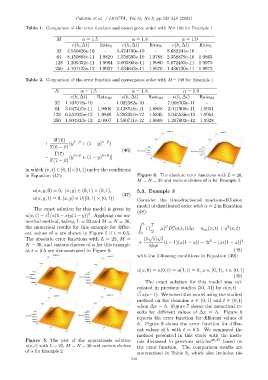
Figure 5. The plot of the approximate solution ods discussed in previous articles 46,47 based on
u(x, t) with L = 20, M = N = 30 and various choices the error function. The comparison results are
of α for Example 2
summarized in Table 3, which also includes the
544