Page 171 - IJOCTA-15-3

A numerical method for solving distributed-order multi-term time-fractional telegraph equations involving
discrepancy between the approximate and exact
solutions, providing a clear indication of the accu-
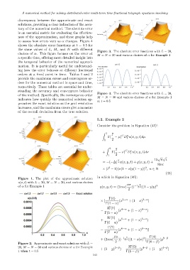
racy of the numerical method. The absolute error
is an essential metric for evaluating the effective-
ness of the approximation, and these graphs help
to assess how errors vary as α changes. Figure 4
shows the absolute error functions at t = 0.5 for
the same values of L, M, and N with different
Figure 3. The absolute error functions with L = 20,
choices of α. This figure focuses on the error at
M = N = 30 and various choices of α for Example 1
a specific time, offering more detailed insight into
the temporal behavior of the numerical approxi-
mation. It is particularly useful for understand-
ing how the error behaves at different fractional
orders at a fixed point in time. Tables 1 and 2
provide the maximum errors and convergence or-
ders for the numerical method in space and time,
respectively. These tables are essential for under-
standing the accuracy and convergence behavior
Figure 4. The absolute error functions with L = 20,
of the method. Specifically, the convergence order
M = N = 30 and various choices of α for Example 1
indicates how quickly the numerical solution ap-
at t = 0.5
proaches the exact solution as the grid resolution
increases, and the maximum errors give a measure
of the overall deviation from the true solution.

5.2. Example 2
Consider the problem in Equation (45)‘:

1 7
Z
µ
C
Γ( − µ) D u(x, y, t)dµ
t
0 2
Z 2 7
C
ν
+ Γ( − ν) D u(x, y, t)dν
t
1 2
√ √
α 15 π t
= −(−∆) 2 u(x, y, t) + g(x, y, t) +
8lnt
2 3
× (t − 1)(x(1 − x)y(1 − y)) , n ∈ N
(45)
in which in Equation (46):
Figure 1. The plot of the approximate solution
u(x, t) with L = 20, M = N = 30, and various choices
απ 5
of α for Example 1 g(x, y, t) = (2cos( )) −1 t 2 ((1 − y)y) 3
2
Γ(4) 3−α 3−α
× [ (x + (1 − x) )
Γ(4 − α)
3Γ(5) 4−α 4−α
− (x + (1 − x) )
Γ(5 − α)
3Γ(6) 5−α 5−α
+ (x + (1 − x) )
Γ(6 − α)
Γ(7) 6−α 6−α
− (x + (1 − x) )]
Γ(7 − α)
βπ −1 5 3 Γ(4) 3−β
+ (2cos( )) t 2 ((1 − x)x) [ (y
2 Γ(4 − β)
Figure 2. Approximate and exact solutions with L =
20, M = N = 30 and various choices of α for Example + (1 − y) 3−β ) − 3Γ(5) (y 4−β + (1 − y) 4−β )
1 when t = 0.5 Γ(5 − β)
543