Page 79 - IJOCTA-15-3

Computational aspects of the crop field segmentation problem based on anisotropic active contour model
f
we define M (·) as a parametrized square ma- 2. Statement of the piecewise-constant
2
f

trix function M (x) = I − η θ(x) ⊗ θ(x) and Mumford–Shah segmentation
demonstrate that the f-decomposition of the do- problem
main Ω relies heavily on this tensor (the technical
details are explained in Section 2). As for the fi- Denote by Ω a bounded open subset of R with
2
delity term T(c, φ), we give its precise definition a Lipschitz boundary. Given a subset E ⊂ Ω, let
in Section 2. Its characteristic feature is the fact |E| be its 2-dimensional Lebesgue measure L (E),
2
that instead of the standard Euclidean metric, we E its closure, ∂E its boundary, and χ E of E the
involve into consideration the Jeffrey divergency characteristic function. The notation u| E denotes
as a more stable metric with respect to outliers.
the restriction of a given function u to the set
The outcomes of simulations using satellite E ⊆ Ω. Indicate the infinitely differentiable func-
∞
photos of agricultural fields, where the area of tions having compact support in Ω by C (Ω).
0
k
high oscillatory edges (the crop locations’ bound- Let H be the Hausdorff k-dimensional measure
aries) is rather significant, support the advantage and µ E the measure µ restricted to the set E.
f
of including M in the final term of J ε . We refer Let f : Ω → R be a given objective function
to Section 4 for further information.
that can be interpreted as a gray-scale image such
0
0
Thus, if (c , φ ) ∈ Absmin J(c, φ), then that a value γ > 0 exists satisfying
(c,φ)∈Ξ ∞
f(x) ≥ γ > 0 a.e. in Ω, f ∈ L (Ω). (2)
Z
1
∗
0
f | (x) = c := f(s) ds, ∀ x ∈ Ω j ,
j
Ω j |Ω j | The following statement for the f-
Ω j
and ∀ j = 0, . . . , m. decomposition of Ω in the framework of the
Mumford–Shah segmentation problem has been
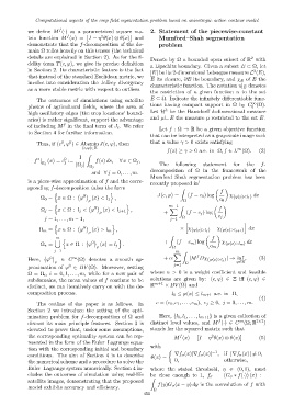
is a piece-wise approximation of f and the corre- 1
recently proposed in
sponding f-decomposition takes the form Z
f
n o J(c, φ) = (f − c 0 ) log χ dx
Ω 0 = x ∈ Ω : φ 0 (x) < l 1 , {φ(x)<l 1 }
ρ Ω c 0
n o m−1 Z
Ω j = x ∈ Ω : l j < φ 0 (x) < l j+1 , X f
ρ + (f − c j ) log
j = 1, . . . , m − 1, j=1 Ω c j
h i
n o
Ω m = x ∈ Ω : φ 0 (x) > l m , × χ {φ(x)>l j } − χ {φ(x)>l j+1 } dx
ρ

f
Z
o
m n
[ 0 + (f − c m ) log χ dx
Ω ∗ = x ∈ Ω : φ (x) = l j . {φ(x)>l m}
ρ Ω c m
j=1
m Z
X f
∞

Here, φ 0 ∈ C (Ω) denotes a smooth ap- + α |M Dχ {φ(x)>l j } | → inf , (3)
ρ Ω φ∈Ξ
0
proximation of φ ∈ BV (Ω). Moreover, setting j=1
Ω = Ω i , i = 0, 1, . . . , m, while for a new pair of where α > 0 is a weight coefficient and feasible
subdomains, the mean values of f continue to be solutions are given by: (c, φ) ∈ Ξ iff (c, φ) ∈
m+1
distinct, we can iteratively carry on with the de- R × BV (Ω) and
composition process. l 0 ≤ φ(x) ≤ l m+1 a.e. in Ω,
(4)
The outline of the paper is as follows. In c = (c 0 , c 1 , . . . , c m ), c j ≥ 0, j = 0, . . . , m.
Section 2 we introduce the setting of the opti-
mization problem for f-decomposition of Ω and Here, {l 0 , l 1 , . . . , l m+1 } is a given collection of
f ∞ 2×2
discuss its main principle features. Section 3 is distinct level values, and M (·) ∈ C (Ω; R )
devoted to prove that, under some assumptions, stands for the squared matrix such that
the corresponding optimality system can be rep- M (x) = I − η θ(x) ⊗ θ(x) (5)
f
2

resented in the form of the Euler–Lagrange equa-
with
tion with the corresponding initial and boundary
−1
conditions. The aim of Section 4 is to describe θ(x) = ∇f σ (x)|∇f σ (x)| , if |∇f σ (x)| ̸= 0,
the numerical scheme and a procedure to solve the 0, otherwise,
Euler–Lagrange system numerically. Section 4 in- where the stated threshold, η ∈ (0, 1), must
cludes the outcomes of simulation using real-life be close enough to 1, f σ = (G σ ∗ f(·)) (x) :=
Z
satellite images, demonstrating that the proposed
f(y)G σ (x − y) dy is the convolution of f with
model exhibits accuracy and efficiency.
Ω
451