Page 172 - IJOCTA-15-4

Oleiwi et al. / IJOCTA, Vol.15, No.4, pp.706-727 (2025)
assigned to each neuron, serves as the input for
these neurons. These weights function similarly
4
to the gains (K p , K i , and K d ) in con-PID con- H(Σ) = − 2 (54)
trol, as shown in Equations (48)–(51). (1 + e −Σ )

P 1 1
where (k) and S (k) are the sum of input con-
i i
nections for each second-layer neuron and the re-
sult of the second layer’s i − th neuron, and vij
and α i represent the weights.
The third hidden layer consists of three neu-
rons. Each neuron in this layer receives weighted
inputs from all outputs of the second hidden layer,
in addition to its previous output and a weighted
contribution from the previous output of the out-
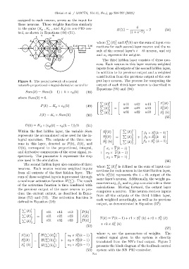
Figure 6. The neural network of a neural put layer neuron. The process for computing the
network–proportional-integral-derivative controller output of each third-layer neuron is described in
Equations (55) and (56):
Sum(k) = Sum(k − 1) + h × e ψ (k) (48)

where Sum(0) = 0.
 
 P 2    1
(k) w11 w12 w13 S (k)
1
P(k) = K p × e ψ (k) (49) P 1 2  1 
2
 (k)  =  w21 w22 w23  S (k)
2  
P 2 1
(k) w31 w32 w33 S (k)
3
I(k) = K i × Sum(k) (50) 3
(55)
D(k) = K d × (e ψ (k) − e ψ (k − 1))/h (51)
Within the first hidden layer, the variable Sum  S (k)   P (k) 2   β 1 × S (k − 1) 
2
2
1
1
1
represents the accumulated value used for the in-  S (k)   P (k)  +  β 2 × S (k − 1) 
2
2
2 
2
2
tegral operation. The outputs of the three neu-  S (k)  =  P 2 β 3 × S (k − 1)
2
2
2
rons in this layer, denoted as P(k), I(k), and 3 (k) 3 3
D(k), correspond to the proportional, integral,  σ 1 × T(k − 1) 
and derivative components of the error signal, re- +  σ 2 × T(k − 1) 
spectively. The parameter h represents the step σ 3 × T(k − 1)
size used in the simulation. (56)
The second hidden layer also consists of three P 2
where (k) is defined as the sum of input con-
neurons. Each neuron receives weighted inputs i
nections for each neuron in the third hidden layer,
from all outputs of the first hidden layer. The while S (k) represents the i − th output of the
2
sum of these weighted inputs is processed through i
P same layer’s neuron. Additionally, the weight pa-
a nonlinear activation function H( ). The result
rameters wij, β i , and σ i play a crucial role in these
of the activation function is then combined with
calculations. Moving forward, the output layer
the previous output of the same neuron to pro-
comprises a neuron. This neuron receives inputs
duce the current output, as described in Equa-
from all the outputs of the third hidden layer,
tions (52) and (53). The activation function is
each weighted accordingly, as well as its previous
defined in Equation (54):
output, as demonstrated in Equation (57):
 P 1 
(k)    
1 v11 v12 v13 P(k)
P
(k)  =  v21 v22 v23   I(k) 
 1 
2
2
 2 T(k) = T(k − 1) + r1 × S (k) + r2 × S (k)
P 1 1 2
(k) v31 v32 v33 D(k)
3 + r3 × S (k)
2
(52) 3
(57)
 1   P 1   1  where r i are the parameters of weights. The
S (k) H( (k) ) α 1 × S (k − 1)
1 1 1 control signal given to the system is directly
S (k)  =  H( α 2 × S (k − 1)
 1   P 1   1 
2
 2 (k) )  +  2  translated from the NN’s final output. Figure 7
1
1
1
S (k) H( P (k) ) α 3 × S (k − 1) presents the block diagram of the feedback control
3
3
3
(53) system with the NN–PID controller.
714