Page 35 - IJPS-7-1

Miladinov

determines h, the minimum segment length allowed when constructing a test (IHS Global Inc., 2017). Small values of
the trimming percentage may lead to estimates of coefficients and variances which are grounded on a very small number
of observations. The optimal number of breaks is based on the sequential methodology. In sequential methodology, the
methods differ in whether the test is performed for a given l breakpoints, for an additional breakpoint in each of the l+1
segments (sequential tests all subsets), or whether the single added breakpoint that most reduces the sum-of-squares
(sequential L+1 breaks vs. L), (IHS Global Inc., 2017). The structural change, the change of the parameters in the sample
period, plays an empirically relevant role in applied time series analysis. In our study, a standard multiple linear regression
model with T periods and m potential breaks (producing m+1 regimes) was considered. For the observations T , T +1.,
j
j
T −1 in regime j, the following regression model has been shown:
j+1
y = X β t ' Z δ + t ' ε + t (1)
t
for the regimes j = 0,…, m. The regressors are divided into two groups. The X variables are those whose parameters do not
vary across regimes, while the Z variables have coefficients that are regime specific. ε is the error term. Once the number
t
and identity of the breakpoints are determined, the model may be estimated using standard regression techniques. The
equation specification above may be rewritten as a standard regression equation:

y = X β t ' Z δ + t ' ε + t (2)
t
 
where β and δ are fixed parameters and δ = (δ 0 ',δ 1 ',… ,δ m ) ' and Z is an expanded set of regressors interacted with
'
t
the set of dummy variables corresponding to each of the m+1 regime segments (IHS Global Inc., 2017). In our research
work, the regression model consists of a regime-specific crude death rate (CDR), TFR, NMR regressors, and a C constant
regressor. The estimated equation is a multivariable regression model in which some of the variables interact with regime
dummy variables. Thus, the equation of the breakpoint model is defined exactly as in the standard least square regression.
In other words, the method used was least squares with breaks. Therefore, dichotomous date functions before, during,
and after a given period are used to generate regime dummy variables that interact with regressors. To the best of the
author’s knowledge, there is no such study that applies the Bai and Perron’s methodology for demographic time series
data. Therefore, this is the motivation for conducting and announcing the results from this research paper.
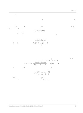
The Bai-Perron test computes the F statistics without structural change (p = 0) on the null hypothesis and p = r when
there are structural changes. If M is a standard matrix, such as (Mλ)’ = (λ’ – λ’ ., λ’ – λ’ ), then
2
r
r+1
1
1 T −  (r + ) 1 q − p  ' ˆ
ˆ
'
'
F β T ( ,… 1 β r ; ) q =   λ M(MV λ ' ˆ ( ) M) Mλ 1 − ˆ (3)
T  rq 
ˆ
where r is breaks, and ( ) λ evaluates the variance-covariance matrix of λ which is robust to serial correlation and
ˆ ˆ
V
heteroskedasticity (Phoong, Phoong, and Phoong, 2020). The breakpoint F-test is given in Equation (4):
[u u −  (uu + u u )/ ] k
'
F = 11 2 2
(uu + 11 u u )/ (T − 2 ) k (4)
2 2
'
where  is the residual of the limited sum of squares, uu is the sum of squared residuals from a sample drawn from
uu
'
j
j
a larger sample j, the number of parameters is denoted with k, and T marks the whole number of observations (Phoong,
Phoong, and Phoong, 2020).
3. Application of A Breakpoint Model for Türkiye: Key Findings
This study provides an empirical approach by applying the method of Bai and Perron from 1998 and 2003 using POPG
rate time series, the CMR, the TFR, and the NMR time series for a sample of Türkiye with data extending over a long
period of 57 years of annual observations. Hence, the task is to identify all breaks in this long time series to ensure that
the breaks in terms of the POPG are accurately and quantitatively identified. Therefore, a breakpoint model was estimated
with POPG regressed on CDR, TFR, NMR, and a constant. The regression output is presented in Table 1.
As can be seen, four statistically significant breaks at 1976, 1984, 2004, and 2013 have been determined using the
Bai-Perron tests of sequentially determined breaks, with a maximum of 5 regimes, 15% trimming, and a test size of 0.05.
Coefficient covariances for the tests and estimates are computed using white estimator with no d.f. correction. Table 1
shows each regime, as well as the corresponding coefficients estimates, standard errors, and p-values. At the bottom of the
table, the standard summary statistics are shown. The results clearly show a significant difference in the mean of CDR,
International Journal of Population Studies | 2021, Volume 7, Issue 1 29