Page 55 - IJPS-9-3

International Journal of
Population Studies Intentional random mathematical model of immigration

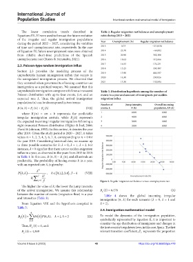
The linear correlation trends described in Table 2. Regular migration net balances and unemployment
Equations III–VI were used to forecast the future evolution rates during 2013 – 2021
of the irregular and regular immigration populations Year Unemployment (%) Regular migration net balance
during the period 2022 – 2027, considering the variables
of time and unemployment rate, respectively. In the case 2013 0.73 −210,936
of Equation IV, future unemployment rates were obtained 2014 23.70 −64,802
from reliable short-time predictions of the Spanish 2015 20.90 383,180
unemployment rate (Torres & Fernández, 2021). 2016 18.63 112,666
2017 16.55 174,231
2.3. Poisson-type random immigration influx
2018 15.25 330,197
Section 2.3 provides the modeling process of the 2019 13.90 444,587
unpredictable human immigration influx that occurs in
the unregulated immigration process. We observed that 2020 16.30 230,026
they occurred when governments of issuing countries use 2021 13.30 153,094
immigration as a political weapon. We assumed that this
unpredictable immigration component follows a truncated Table 3. Distribution hypothesis among the number of
Poisson distribution with up to four events, J=4, and an events in a year and amount of immigrants per sudden
expected rate . Thus, the global arrival immigration migration influx
population () can be decomposed in two terms:
Number of Jump intensity, Overall incoming
B (n, λ) = B (n) + B (λ) (VII) events, k N (k) population, kN (k)
1 2
where () = + represents the predictable 1 6000 6000
1
irregular immigration arrivals, while () represents 2 4000 8000
2
the expected incoming irregular immigration following a 3 3000 9000
right-truncated Poisson distribution (Yiğiter & İnal, 2006; 4 2000 8000
David & Johnson, 1952). In this context, denotes the year
after 2019. Given the study period is 2020 – 2027, takes
values = 1, 2, 3, 4, 5, 6, 7, 8, corresponding to = 0 for
the year 2019. Considering historical data, we assume up
to three possible scenarios for : = 0, = 1, = 2. For
instance, = 0 signifies that there are no sudden migration
influx in a year, as observed in the years from 2013 to 2018
in Table 1. In this case, (, 0) = (), and all arrivals are
1
predictable. The probability of having events in a year,
with an expected rate , is given by:

Pk, k j , k012 J , 4 (VIII)
, ,, ,34
k! J Figure 3. Regular migration net balance versus unemployment rate.
j!
j0
The higher the value of , the lower the jump intensity
of the arrival immigration. We assume this relationship B (2) = 6,476 (X)
2
between the number of events (migration flow) in a year Table 4 shows the global incoming irregular
and intensities (Table 3). immigration (, ) for each scenario ( = 0, = 1 and
From Equation VIII and the hypothesis compiled in = 2).
Table 3:
2.4. Immigration mathematical model
4

B kNk Pk (, ), 1 , 2 (IX) To model the dynamics of the immigration population,
2
k 0 symbolically represented by Equation II, it is important to
Thus, (0) = 0, and: consider the age distribution of immigrants and changes in
2 the host country’s regulatory laws, in this case, Spain. The first
B (1) = 4,369 relevant transition coefficient, , represents the proportion
2 1

Volume 9 Issue 3 (2023) 49 https://doi.org/10.36922/ijps.478