Page 83 - MSAM-1-1

Materials Science in Additive Manufacturing A ML model for AM PSP of Ti64

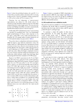
Figure 5 shows the individual variance for each PC. It is Figure 6 shows an example of EBSD observation on
evident that cumulative variance increases with increasing the heat-treated L-PBF XY plane sample and Table S1 in
numbers of PCs. The PCA cumulative variance approaches the Supplementary File shows the average SF at different
to >99% as the number of PCs increases to 238. slip systems and Taylor factor of different strain rates for
Therefore, the total dimension of microstructural different AM material surfaces.
representation was reduced to 238, which reduces the 3.2. ML model and cross-validation results
dimension of the descriptor matrix by more than 92% when
compared with the original input matrix. This was critical to The goal of this study to establish the S-P linkage by training
develop an SP linkage model that was both computationally a regression ML model relies on machining parameters,
feasible and accurate to predict material response. microstructure functions, residual stress, and SF input to
predict the specific cutting energy.
In this study, XRD residual stresses were measured along
the direction of machining feed. The X-ray penetration To construct a robust ML model, the first step is
depth varied between 25~50 µm, which depends on the data preparation. In this study, the dataset contains
tilt angles. Using XRD crystal strain measurements and 14,400 sample points with 72 different machining
Equation (II), the average surface residual stresses for all parameter combinations and 200 sets of microstructure
six AM material surfaces are presented in Table 2. data for every AM material surface. After PCA of the SEM
microstructure, this was reduced to one response variable
The positive value in residual stress indicates tensile stress, (specific cutting power) and 262 features: 238 features
while the negative value indicates compression stress. The for PCA processed features to represent microstructure
residual stress on L-PBF surfaces after heat treatment shows function, three features for the residual stress, nine features
a decrease in shear stress. However, heat treatment does not for SFs input, nine features for the Taylor factors input, and
heavily influence the near-surface crystal principal stress in three features for the machining parameter combinations
Y and Z directions in L-PBF specimens. EB-PBF samples (feed, speed, and depth of cut). For each machining
as-AM top surface shows the largest compressive stress in parameter combination, three replicates were conducted,
the Y-axis direction and the smallest principal stress in the and the average specific cutting energy was treated as the
Z-direction, which indicates tensile stress and large shear response variables.
stress along with the build orientation in EB-PBF sample.
The next step is to train a regression model (random
Based on the EBSD measurements, the SF and Taylor
factor (M values) were calculated from crystal orientation 80% dataset) for testing (20% dataset). This study
employed XGBoost (eXtreme Gradient Boosting Tree-
distribution using MATLAB program. Average SF and M based approach) and linear regression models for training.
values for each SVE were added to the PCA descriptor Chen and Guestrin (2016) presented the XGBoost
matrix. Zhang et al. (2019) indicated that the SF analysis model, which has been widely used due to its accuracy
shows SVE with high variants of active twinning and [28]
detwinning should have high values of SF . Considering and interpretability . XGBoost is a regularized gradient
[19]
the major slip systems in α-Ti-6Al-4V, basal, prismatic, boosting machine which controls for overfitting by
and the first-order pyramidal slip systems were applied employing a more regularized objective function that
in the Schmid model, while the critical resolved shear incorporates both a convex loss function and a penalty
stress (CRSS) ratio for these selected three slip systems is parameter for regression tree function. The classical linear
1:0.7:3. Demir (2009) showed that the deformation strain regression model is used as the baseline model. Both models
(DS) in Taylor factor calculation for a peripheral milling were implemented using Sklearn packages in Python. A grid
process can be expressed as a sum of pure shear and search approach for tuning the hyperparameters, including
angular shear, as shown in Equation (XII) . Since the the maximum depth of each subtree and the number of
[41]
strain varies based on the machining parameters, three subtrees, was applied. A grid search evaluates different
different strain rates were selected in the Taylor model combinations of hyperparameters by cross-validation and
calculation. selecting the best hyperparameter set to train the estimator
of a learning model. During validation, the test set (20%)
was applied to the best XGBoost estimator and the linear
0 0 0 0 model to validate their accuracies with the root mean
2 2 square error (RMSE) being the evaluation metric for the
DS 0 0 0 0 0 0 (XII) accuracy of the ML model.

0 0 0 0 To better understand the influence of machining
2 2 parameters, microstructure functions, residual stress,

Volume 1 Issue 1 (2022) 11 https://doi.org/10.18063/msam.v1i1.6