Page 85 - MSAM-4-3

Materials Science in Additive Manufacturing Interpretable GP melt track prediction

A

B

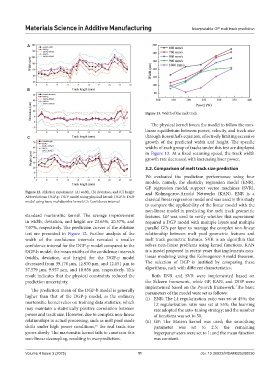
Figure 13. Width of the melt track

The physical kernel forces the model to follow the non-
linear equilibrium between power, velocity, and track size
C through Rosenthal’s equation, effectively limiting excessive
growth of the predicted width and height. The specific
widths of each group of tracks under this test are displayed
in Figure 13. At a fixed scanning speed, the track width
growth rate decreased with increasing laser power.

3.2. Comparison of melt track size prediction
We evaluated the prediction performance using four
models, namely, the elasticity regression model (ENR),
GP regression model, support vector machines (SVR),
Figure 12. Ablation experiment: (A) width, (B) deviation, and (C) height and Kolmogorov-Arnold Networks (KAN). ENR is a
Abbreviations: DGP-p: DGP model using physical kernel; DGP-b: DGP classical linear regression model and was used in this study
model using basic mahalanobis kernel; CI: Confidence interval
to compare the applicability of the linear model with the
non-linear model in predicting the melt track geometric
standard martensitic kernel. The average improvement features. GP was used to verify whether this experiment
in width, deviation, and height are 23.65%, 20.57%, and required a DGP model with multiple layers and multiple
7.07%, respectively. The prediction curves of the ablation parallel GPs per layer to manage the complex non-linear
test are presented in Figure 12. Further analysis of the relationship between melt pool geometric features and
width of the confidence intervals revealed a smaller melt track geometric features. SVR is an algorithm that
confidence interval for the DGP-p model compared to the solves non-linear problems using kernel functions. KAN
DGP-b model; the mean widths of the confidence intervals is a model proposed in recent years that implements non-
(width, deviation, and height) for the DGP-p model linear modeling using the Kolmogorov-Arnold theorem.
decreased from 39.170 μm, 12.970 μm, and 12.051 μm to The selection of DGP is justified by comparing these
37.579 μm, 9.957 μm, and 10.858 μm, respectively. This algorithms, each with different characteristics.
result indicates that the physical constraints reduced the Both ENR and SVR were implemented based on
prediction uncertainty. the Sklearn framework, while GP, KAN, and DGP were
implemented based on the Pytorch framework. The basic
The prediction mean of the DGP-b model is generally parameters of the model were set as follows:
higher than that of the DGP-p model, as the ordinary (i) ENR: The L1 regularization ratio was set at 45%; the
martensitic kernel relies on training data statistics, which L2 regularization ratio was set at 55%; the learning
may maintain a statistically positive correlation between rate adopted the auto-tuning strategy; and the number
power and track size. However, due to complex non-linear of iterations was set to 50.
relationships in actual processing, such as melt pool mode (ii) GP: The Matérn kernel was used; the smoothing
shifts under high power conditions, the real track size parameter was set to 2.5; the remaining
16
grows slowly. The martensitic kernel fails to constrain this hyperparameters were set to 1; and the mean function
non-linear decoupling, resulting in overprediction. was constant.

Volume 4 Issue 3 (2025) 11 doi: 10.36922/MSAM025200030