Page 86 - MSAM-4-3

Materials Science in Additive Manufacturing Interpretable GP melt track prediction

(iii) SVR: The radial basis kernel function was used and From the model RMSE results, the DGP – optimized
the regular term coefficient was set to 1. based on the physical model – significantly outperformed
(iv) KAN: Three hidden layers were used; the number of the GP, KAN, SVR, and ENR models in the prediction
neurons was 36, 24, and 12, respectively, connected of melt track geometric features. To further elucidate the
by fully connected form; the number of iterations was rationale for selecting the DGP model, the 340 W-960 m/s
100; the optimizer used Adam; and the learning rate experimental set with the largest RMSE index was further
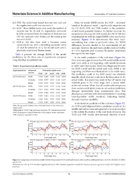
was set to 0.001. analyzed. Figures 14-16 demonstrate that when back-
(v) DGP-p: The first layer used a Gaussian cosine normalizing true values to predicted values, the RMSE
composite kernel, with a smoothing parameter set to differences between models in the experimental set are
2.5 and the period set to 1; the second layer used a minimal. However, the melt track exhibits reduced widths
physically constrained Matérn kernel. in initial segments and increased fluctuation amplitudes
Table 2 presents the average RMSE of the model during mid-to-late stages.
predictions for the three sets of experiments computed In the width prediction of the melt track (Figure 14),
using MinMax-normalized data. there were some gaps between the SVR model and the actual
melt track width at the beginning, with notable hysteresis
Table 2. Experimental prediction results at width value fluctuations. There was a bigger gap between
the KAN model and the actual melt track width at the
Experimental set Geometric Root mean square error beginning, and there were fluctuations in the width value.
features DGP GP KAN SVR ENR The prediction result of the ENR model was relatively

240 W-660 mm/s Width 0.060 0.288 0.268 0.236 0.234 smooth, which does not conform to the fluctuation of the
Deviation 0.020 0.097 0.057 0.124 0.150 actual width. The prediction result of the GP model was
Height 0.043 0.053 0.047 0.048 0.048 relatively good in the initial stage, with a decent width
290 W-760 mm/s Width 0.065 0.170 0.157 0.136 0.141 in the tail section. While the GP model achieved precise
Deviation 0.017 0.121 0.032 0.044 0.045 front-section width predictions, its tail-section predictions
diverged substantially from experimental data. This
Height 0.036 0.062 0.050 0.054 0.044 discrepancy correlates with observed hysteresis in tracking
340 W-960 mm/s Width 0.083 0.201 0.174 0.136 0.151 time-dependent width variations, indicating limited
Deviation 0.024 0.041 0.055 0.049 0.045 dynamic response capability.
Height 0.038 0.067 0.069 0.052 0.061 In the deviation prediction of the melt track (Figure 15),
Note: The geometric features were evaluated based on the root mean the SVR model displayed better prediction results in the
square error. middle and end sections and appeared to be more sensitive
Abbreviations: DGP: Deep Gaussian processes; GP: Gaussian processes;
KAN: Kolmogorov-Arnold Networks; SVR: Support vector machines; to the sudden fluctuation of the melt track deviation. The
ENR: Elasticity regression model. KAN and ENR models demonstrated relatively smooth

A B

C D

Figure 14. Comparison of validation results between the proposed DGP model and various other models in width prediction: (A) SVR, (B) KAN, (C) ENR,
and (D) GP
Abbreviations: DGP-p: DGP model using physical kernel; ENR: Elasticity regression model; GP: Gaussian process regression model; SVR: Support vector
machines

Volume 4 Issue 3 (2025) 12 doi: 10.36922/MSAM025200030