Page 83 - MSAM-4-3

Materials Science in Additive Manufacturing Interpretable GP melt track prediction

Finally, the geometrical parameter height, and position (Equations XIX-XXII).
t ∑
() 2
1 ()
1 ()’
Y = 6 j=1 w K ( F , F ) of the output melt track of the Δ = [ΔV, ΔW, ΔD, ΔH] (XIX)
j
j
second layer. ΔW = W t–W (XX)
The DGP-p model in this study was trained using
variational inference combined with stochastic gradient ΔD = D t–D (XXI)
descent. Unlike traditional GP, the multilayer structure of ΔH = H t–h (XXII)
DGP limits the direct computation of the exact posterior Where ΔW, ΔD, and ΔH denote the deviations in melt
distribution. Hence, the variational inference was used track width, deviation, and height, respectively.
to approximate the posterior distribution. The objective
Based on the deviation features and melt track category
function of the model is the evidence lower bound (ELBO). labels, a simple and efficient softmax classifier was utilized
( ) 1
( ) θ = E q  L  ( |y F (2) ) logp  −   ( ) || (p F ( ) 1 | X t )   − KL q F to classify the melt track categories.
(

KL q F ( ) 2 |F ( ) 1 ) || (p F ( ) 2 |F ( ) 1 )  (XVII) 2.6. Model training
 
During training, the root mean square error (RMSE)
Where θ denotes the model learnable parameter. (Equation XXIII) was used to evaluate model performance.
θ is all learnable parameters.
E q [logp(y|F )] is the expected log-likelihood of y with  1 n 2  05.
(2)
i ( ∑
f
given F . RMSE =  f − )  (XXIII)
(2)
i
q(F ) isthe variational distribution of hidden variables  n i=1 
(1)
in the first layer. Where n is the number of samples, f is the true value,
q(F /F ) is the conditional variational distribution of and f i is the predicted value. i
(1)
(2)
second-layer hidden variables given F .
(1)
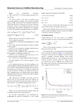
p(F |X t) is the conditional prior distribution of the The training effect of the proposed model using RMSE
(1)
loss in 70 epochs is displayed in Figure 10. During the first
first-layer latent variable given the input X t
p(F |F ) is the conditional prior distribution of the 10 epochs, both training and validation losses decreased
(2)
(1)
second-layer latent variable given F . rapidly in parallel, indicating efficient initial model
(1)
KL(·): This function means kullback-leibler divergence. learning. Between epochs 10 – 40, convergence decreased
We using Equation XVII as the loss equation to train without oscillation. Beyond epoch 40, while training
the model. loss continued to decline, validation loss exhibited slow
fluctuations with a gradually widening divergence between
In the optimization process, the Adam optimizer was them, suggesting mild overfitting.
used for gradient updating. The initial learning rate was set
to 0.01, and an exponential decay strategy was used, where
the learning rate was decayed to 0.9 times the original rate
at every 50 rounds of iterations. To avoid local optima, an
early stopping strategy was implemented during training,
halting the process when the validation loss fails to improve
over 10 consecutive epochs.
After obtaining the predicted melt track geometric
features [W t, D t, H t] from the melt pool features, the
deviation of the predicted melt track volume Vol t from the
ideal volume V was calculated using Equation XVIII.
 πW 2 1 
= V t − Vol =Vol  ∆  t − W H t  L 2 +  t −(D D t −1 2 − ) V
t
 4 2 
(XVIII)
Where L v is the corresponding track length of the melt
pool under different laser scanning speeds.
The deviation characteristics were determined by Figure 10. Root mean square error loss of the DGP-p model
synthesizing the predicted deviations of track width, Abbreviations: DGP-p: DGP model using physical kernel; Val: Validation
datasets; Train: Training datasets

Volume 4 Issue 3 (2025) 9 doi: 10.36922/MSAM025200030