Page 117 - AJWEP-22-6

SWAT-based LULC impacts on groundwater recharge

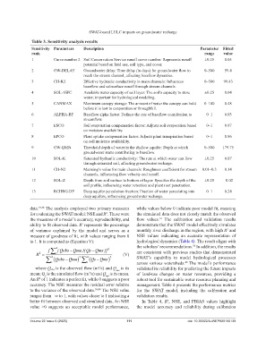
Table 3. Sensitivity analysis results
Sensitivity Parameters Description Parameter Fitted
rank range value
1 Curve number 2 Soil Conservation Service runoff curve number: Represents runoff ±0.25 0.05
potential based on land use, soil type, and cover.
2 GW-DELAY Groundwater delay: Time delay (in days) for groundwater flow to 0–500 59.4
reach the stream channel, affecting baseflow dynamics.
3 CH-K2 Effective hydraulic conductivity in main channels: Influences 0–500 99.43
baseflow and subsurface runoff through stream channels.
4 SOL-AWC Available water capacity of soil layer: The soil’s capacity to store ±0.25 0.04
water; important for hydrological modeling.
5 CANMAX Maximum canopy storage: The amount of water the canopy can hold 0–100 0.48
before it is lost to evaporation or throughfall.
6 ALPHA-BF Baseflow alpha factor: Defines the rate of baseflow contribution to 0–1 0.03
streamflow.
7 ESCO Soil evaporation compensation factor: Adjusts soil evaporation based 0–1 0.97
on moisture availability.
8 EPCO Plant uptake compensation factor: Adjusts plant transpiration based 0–1 0.96
on soil moisture availability.
9 GW-QMN Threshold depth of water in the shallow aquifer: Depth at which 0–500 179.75
groundwater starts contributing to baseflow.
10 SOL-K Saturated hydraulic conductivity: The rate at which water can flow ±0.25 0.07
through saturated soil, affecting groundwater recharge.
11 CH-N2 Manning’s value for main channels: Roughness coefficient for stream 0.01–0.3 0.14
channels, influencing flow velocity and runoff.
12 SOL-Z Depth from soil surface to bottom of layer: Specifies the depth of the ±0.25 −0.02
soil profile, influencing water retention and plant root penetration.
13 RCHRG-DP Deep aquifer percolation fraction: Fraction of water percolating into 0–1 0.24
deep aquifers, influencing groundwater recharge.

data. 37,38 The analysis employed two primary measures while values below 0 indicate poor model fit, meaning
for evaluating the SWAT model: NSE and R . These were the simulated data does not closely match the observed
2
the measures of a model’s accuracy, reproducibility, and flow values. The calibration and validation results
37
ability to fit observed data. R represents the percentage demonstrate that the SWAT model effectively simulates
2
of variance explained by the model and serves as a monthly river discharge in the region, with high R and
2
measure of goodness of fit, with values ranging from 0 NSE values indicating an accurate representation of
to 1. It is computed as (Equation V): hydrological dynamics (Table 4). The result aligns with
the scholars’ recommendations. In addition, the results
38
n
[ ( Qobs QmoQs Qms )( )] 2 are consistent with previous studies that demonstrated
2
R i (V)
n i Qobs Qmo 2 n i Qs Qms 2 SWAT’s capability to model hydrological processes

across various watersheds. The model’s performance
49
where Q obs is the observed flow (m³/s) and Q is its validated its reliability for predicting the future impacts
mo
mean; Q is the simulated flow (m /s) and Q is its mean. of land-use changes on water resources, providing a
3
ms
s
An R of 1 indicates a perfect fit, while 0 suggests a poor robust tool for sustainable water resource planning and
2
accuracy. The NSE measures the residual error relative management. Table 4 presents the performance metrics
to the variance of the observed data. 38,48 The NSE value for the SWAT model, including the calibration and
ranges from −∞ to 1, with values closer to 1 indicating a validation results.
better fit between observed and simulated data. An NSE In Table 4, R , NSE, and PBIAS values highlight
2
value >0 suggests an acceptable model performance, the model accuracy and reliability during calibration
Volume 22 Issue 6 (2025) 111 doi: 10.36922/AJWEP025180139