Page 88 - DP-2-1

Design+ Analysis of 3D-printed anisotropic cells

Probes were also defined to measure reaction forces and ε  
deformations (normal and shear) of cell units as a function  x 
of the displacement. Therefore, it is possible to identify the  ε x 
correlation between average stresses and the deformation ε  
of cell units.  x 
Multiple steps were applied to characterize the  γ yz  =
orthotropic elasticity and shear moduli of unit cells, with a   γ xz  
step increment was 0.001 mm. Therefore, we can consider  γ xy 
these studies as Dirichlet-Dirichlet problems.  
It is also possible to note that the deformation in all  
directions (εx, εy, εz, γxy, γxz, γzy) and the maximum  1 − v xy − v 
equivalent stress (von Mises) were acquired in each step,  E E E xz 0 0 0 
allowing the calculation of the elastic and shear moduli for  x x x 
the unit cell in each step. By the end, the average moduli  v xy 1 − v yz  −
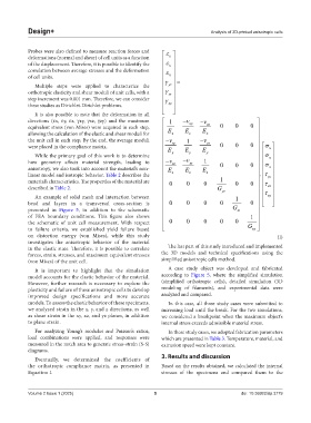
were placed in the compliance matrix.  0 0 0  σ  x 
 E y E y E y   
While the primary goal of this work is to determine    σ x 
how geometry affects material strength, leading to  − v xz − v yz 1 0 0 0  σ  
anisotropy, we also took into account the material’s non-  E E E   x 
linear model and isotropic behavior. Table 2 describes the  z z z  . τ yz 

material’s characteristics. The properties of the material are  0 0 0 1 0 0   τ 
described in Table 2.  G yz   xz 
An example of solid mesh and interaction between   1     τ xy  
bead and layers in a transversal cross-section is  0 0 0 0 0   
presented in Figure 5, in addition to the schematic  G xz 
of FEA boundary conditions. This figure also shows  1 
the schematic of unit cell measurement. With respect  0 0 0 0 0 G 
to failure criteria, we established yield failure based  xy 
on distortion energy (von Mises), while this study (I)
investigates the anisotropic behavior of the material
in the elastic state. Therefore, it is possible to correlate The last part of this study introduced and implemented
forces, strain, stresses, and maximum equivalent stresses the 3D models and technical specifications using the
(von Mises) of the unit cell. simplified anisotropic cells method.
It is important to highlight that the simulation A case study object was developed and fabricated
model accounts for the elastic behavior of the material. according to Figure 5, where the simplified simulation
However, further research is necessary to explore the (simplified orthotropic cells), detailed simulation (3D
plasticity and failure of these anisotropic cells to develop modeling of filaments), and experimental data were
improved design specifications and more accurate analyzed and compared.
models. To assess the elastic behavior of these specimens, In this case, all three study cases were submitted to
we analyzed strain in the x, y, and z directions, as well increasing load until the break. For the two simulations,
as shear strain in the xy, xz, and yz planes, in addition we considered a breakpoint when the maximum object’s
to plane strain. internal stress exceeds admissible material stress.
For analyzing Young’s modulus and Poisson’s ratios, In these study cases, we adopted fabrication parameters
load combinations were applied, and responses were which are presented in Table 3. Temperature, material, and
measured in the notch area to generate stress-strain (S-S) extrusion speed were kept constant.
diagrams.
3. Results and discussion
Eventually, we determined the coefficients of
the orthotropic compliance matrix, as presented in Based on the results obtained, we calculated the internal
Equation I. stresses of the specimens and compared them to the

Volume 2 Issue 1 (2025) 5 doi: 10.36922/dp.3779