Page 91 - DP-2-1

Design+ Analysis of 3D-printed anisotropic cells

A physical object often contains porosities. These porosities
lead to a reduction in the actual density of the object, which
varies depending on the layer height and filament diameter.
In Figure 8, the contour diagram shows the overlap of
parameters that leads to the best results for each response.
The feasible area represents the combination of factors that
produce maximum mechanical strength. Objects made with
thicker layers demonstrate the highest mechanical strength,
particularly when the line overlap is moderate and the bead
width is high. In addition, it is evident that beyond a certain
level of overlap, further increases do not significantly enhance
mechanical strength. This can be attributed to the fact that, past
a certain point, the porosity does not decrease significantly.
B This study provides a predictive framework for
understanding the mechanical behavior of objects fabricated
with raster cells. It serves as a valuable tool for engineers and
designers to accurately specify the mechanical strength of
entire objects or specific components in technical drawings.
In addition, this approach ensures consistent quality and
repeatability of mechanical and dimensional properties
regardless of the manufacturing site.
Regarding raster cells, we identified the linear
orthotropic compliance matrix as a function of control
factors, as presented in Equation II. This matrix was
developed in order to create simplified finite element
models that can simulate objects with variable anisotropic
C behavior at a low computational cost.

  + 0.2894   + 0.06005  − 0.0038 0.01075 O− ⋅  
  0.09 O  ⋅  − 0.0198 O  ⋅  + 0.033 Wd⋅  
  − −  0.2889 h⋅     − 0.0747 h⋅     + 0.188 h⋅   0 0 0  
        0.191.Wd h⋅   
    −   
  + 0.148  
 + 0.0505   + 1.25 O  + 0.01011  
⋅
     0 0 0 
  0.0789 h  − ⋅  + 0.291 h ⋅   0.0672 h  + ⋅  
  − ⋅ ⋅  
  7.36 Wd O  
 + 0.081 0.588 O− ⋅  
 0.160 Wd⋅    + 0.1085   + 0.419  
 −    0.471 h  −  ⋅ − 2.01 h⋅   
 −  0.507 h⋅      0 0 0 
 1.302 Wd O⋅ ⋅      − 0.265 Wd⋅  − 0.842 Wd⋅  
  −  1.586 Wd h  +  ⋅ ⋅     + 1.89 Wd h⋅ ⋅     + 6.19 Wd h⋅ ⋅    
  C=    − 0.786   
   + 6.13 h ⋅   
 0 0  .1.91 Wd  0 0 
⋅
 
   − 10.44 Wd h ⋅ ⋅   
 
 + 0.901 7.23 O 
⋅
−
  − 1.241 Wd  
⋅
   
  − 2.527 h ⋅  
 0 0 0 0   0 
 +  8.25 Wd O  ⋅ ⋅ 
  17.53 O h  + ⋅⋅ 
   
 +  4.84 Wd h ⋅ ⋅  
 
   − 2.24   
12.83 h ⋅
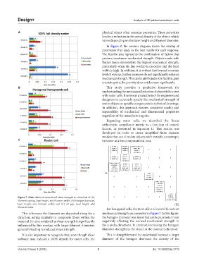
Figure 7. Main effects of normal and shear strength as a function of (A)    0 0 0 0 0   − + 5.14 Wd     
⋅

filament overlap, layer height, and filament width; (B) hexagon diameter,     − 28.4028 Wd h ⋅ ⋅   
layer height, and filament width; and (C) air gap, layer height, and (II)
filament width.
For hexagonal cells, the main effect of control factors on
This is because the filaments are deposited along the y mechanical strength are presented in Figure 7. In this figure,
direction, acting similarly to composite fibers within the the hexagon diameter was identified as the parameter most
material. It is also evident that shear strength is significantly negatively affecting the normal mechanical strength in
influenced by line overlap, with larger filament diameters the x and y directions. In contrast, increasing the hexagon
generally leading to reduced shear strength. diameter strengthens the object in the normal z direction.
It is also important to recognize that, even though slicer This is straightforward to understand because a larger
software may indicate a 100% density for raster cells, the diameter of the hexagon decreases the density of the
Volume 2 Issue 1 (2025) 8 doi: 10.36922/dp.3779